While calibrations are covered in detail in another section of the measurement guide, there are some peculiarities relative to broadband and mm-Wave operation that require some comment.
• The mm-Wave bands are often executed in waveguide thus requiring that media type selection (to take care of dispersion correction).
• SOLT/SOLR are often not recommended due to the difficulty of fabricating a reasonable open standard. An open waveguide flange radiates quite effectively and, as a result, is both unstable and has a relatively high return loss.
• SSLT/SSLR are commonly used, particularly at lower frequencies and do require a good load standard. The offset short lengths must be known with some precision.
• SSST/SSSR is quite popular, particularly at higher frequencies since a load standard is not required. Accurate knowledge of the short offset lengths is critical.
• LRL is also a popular technique and is quite effective although it can be sensitive to the condition of the waveguide flanges.
Classical BB Mode
In classical broadband mode, a hybrid coupler combining the bands into a single W1 coaxial connector is typically used with a default breakpoint of 67 GHz (i.e., at 67 GHz and below, the base VNA is used for both source and receiver; at 67.000000001 GHz and above, the external modules are used for source and receiver). This structure is key to allowing the combined sweep. To calibrate this connector type, typically two calibrations are recommended: SOLT from the low frequency limit to 67 GHz and SSST from 67-110 GHz. The two calibrations are performed separately and then combined using cal merge (see calibration section for details). The only constraints are the two calibrations must be of the same type (i.e., both 1-Port S11 or both full 2-Port) and the total point count must not exceed the current maximum for the instrument (25000 or 100000). Note that other calibration types (e.g., LRL) can be successfully combined with this connector type.
Note
It is important that the system be in the appropriate 3739 receiver configuration even when performing the lower frequency calibration. This ensures that the correct receiver mode is used in the merged calibration.
In the 3739-based systems, a similar protocol is used with a 67 GHz breakpoint also typically used for ME7838A (and related) systems (W1 connector-based). For the ME7838D and related systems (using the MA25300A modules) which are 0.8 mm-connector based, a breakpoint for the calibrations of 80 GHz is typically used. In all cases, it is generally an SOLT calibration at the lower frequencies and an SSST calibration at higher frequencies.
The 1mm (W1) and 0.8 mm calibration kits both contain 3 shorts, an open, and a load for both connector genders (along with many adapters, tools and verification components). For the SOLT calibration, the coefficients are setup assuming that SHORT 1 is used for that calibration.
Modular BB Approach
In the modular BB approach, the multiplexing is instead done behind the high frequency reflectometers and happens at two disjoint frequencies instead of at a common breakpoint. This typically does not affect the calibration break frequency as the latter is more determined by the characteristics of the calibration kit. Thus when using Anritsu’s 3656B W1 calibration kit, the same 67 GHz breakpoint is commonly used for both the classical and modular broadband systems.
Some additional comments related to use of the modular BB system:
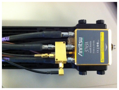
• Since the thru path of the modules is DC-connected, the internal VNA bias tees can be used (the bias routes from the VNA rear panel through the VNA front panel ports to the modules, and then to the W1 plane). For Kelvin-based measurements, Anritsu Kelvin bias tees can be mounted on the rear of the modules directly (see Figure: The connection of a Kelvin bias tee to a mm-wave module is shown here.). A variety of bias tees are available with different video bandwidths and current handling capabilities are available; contact Anritsu for more information. The internal DC resistance of the modules is very low so the drop from the bias tee to the DUT can be minimized. Contact Anritsu for a detailed report.
• Because the bias tees often have 70 GHz bandwidth and are very well matched, they have little impact on system raw directivity, in part because they are positioned behind the high frequency couplers.
The connection of a Kelvin bias tee to a mm-wave module is shown here.
• Isothermal measurements are often of interest and the position of the module very close to the reference plane sometimes raises the question of thermal effects. When normally mounted, the temperature rise at a wafer probe tip is less than 1 degree C. If even low temperature rises are required for on-wafer or other applications, mounting variations are available to reduce this rise to under 0.3 degree C (about the limit of the thermometry being used). Contact Anritsu for more information.
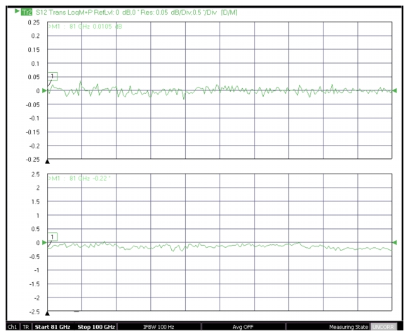
• It is sometimes desirable to position the modules remotely (or further than the usual 1 m cables would allow) because of a complex test setup or for antenna measurement and other applications. Up to 5 m cable runs can be used with reasonable performance (power and dynamic range below 54 GHz will be affected by insertion loss changes, but mm-wave performance will not be because of saturating mixers and multipliers) and 15 m cable runs can be used in some circumstances (covering 30-125 GHz for the 3743A module). For information on configuring longer cable sets or for special modifications for even more remote applications, contact Anritsu. Trace noise and short term stability from measurements with a 15 m system are shown in Figure: Trace noise and stability over about 1 hour are shown here for a 15 m antenna-based measurement.. This measurement was done with conventional horn antennas in a laboratory environment and mainly serves to show reasonable close-in trace performance with long cable runs.
Trace noise and stability over about 1 hour are shown here for a 15 m antenna-based measurement.
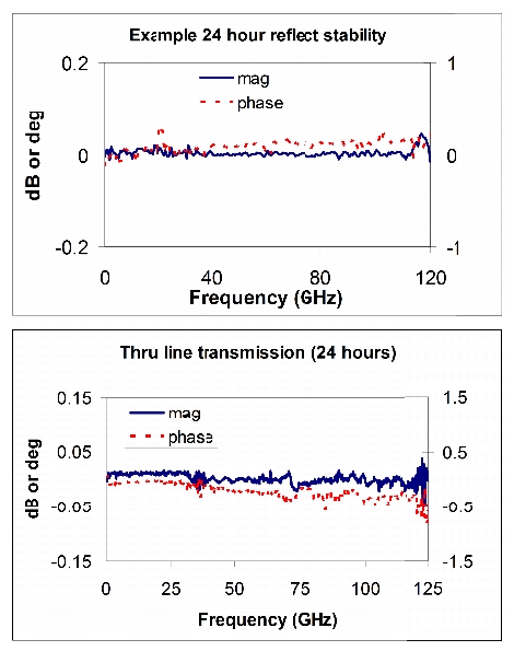
• In broadband and mm-wave measurements, stability is often of interest because of the possibility of long measurement sessions or longer calibrations. It would be desirable if a calibration could last for a longer period of time to reduce the chance of invalid measurements and to reduce the overall time spent calibrating. The modular BB approach offer some advantages in having the high frequency couplers (covering 30-145 GHz) being right at the 1 mm (or 0.8 mm) connector to minimize raw directivity degradation, a small integrated package to avoid thermal gradients, and a tightly integrated control system. The result is good stability in both reflection and transmission over time as suggested in Figure: Stability data for the modular BB system.. In order to optimize stability, minimizing environmental temperature variations certainly helps as does protecting the cable runs from overstress or unnecessary exposure to thermal variation.
Stability data for the modular BB system.
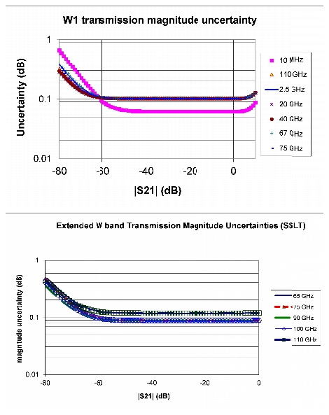
• Waveguide-based measurements are sometimes needed. The classical approach can simply demount the mux coupler and use the exposed waveguide flange (WR-10, 75-110 GHz in that case). A variety of adapters are available for the modular BB approach in WR-15, WR-12, and WR-10 sizes (50-75, 60-90, and 75-110 GHz nominal, respectively). A bracket comes with these adapters to prevent stress from being applied to the 1 mm connector and to improve measurement repeatability. Waveguide calibration kits (3655 series) are available to support SSLT and LRL calibrations referenced to these waveguide planes. The uncertainties do not differ markedly between coaxial and waveguide-based calibrations in these bands as suggested in Figure: Example coaxial and waveguide uncertainty curves are shown here., but the waveguide measurements can be more subject to repeatability issues depending on the physical setup and flange quality on the DUT or on any extensions (some high quality extensions are included in the calibration kits to help with the latter).
Example coaxial and waveguide uncertainty curves are shown here.