Final topics for this chapter are some ancillary measurements.
Spurs
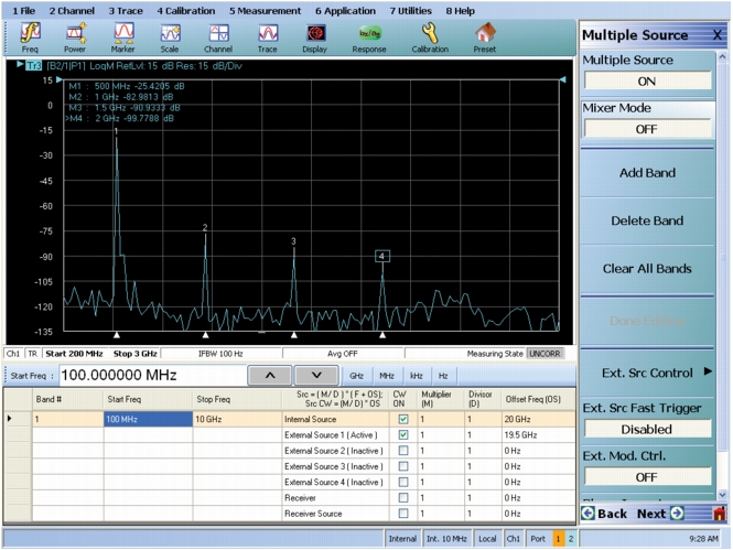
The MS464XX can be used as a spectrum monitor to scan for spurious products of the mixer. This is most easily done with multiple source control (see Multiple Source Control (Option 007)) with the input source and LO usually set to some CW frequencies and the receiver allowed to sweep over a range of interest to look for spurious products on the LO. The unratioed test channel is often used as a monitor and a receiver calibration can be applied to get an absolute signal level for those spurious products. An example setup is shown in Figure: Multiple Source Setup – Search for Spurious Products where the source is parked at 20 GHz and LO at 19.5GHz. The desired IF is 0.5 GHz but we can sweep over a wider range to look for products and the result is shown in the figure as well.
In this particular case (and with the sweep resolution used here), the dominant spurs are all harmonics of the IF. Using the previous nomenclature, they are of the form N × (Input – LO) and they are all at least 55 dB below the desired IF. With a different sweep range and point density, other spurs might have been found so it does help to work out the frequency plan in advance where likely spurs might reside.
Multiple Source Setup – Search for Spurious Products
A multiple source setup to look for spurious products on an example DUT is shown here. The plot shows the products measured,
One does have to exercise some caution in interpreting these results since the VNA receiver is not pre-selected and there may be internally generated spurs as well. In addition, the internal converters have an image located (usually) 24.7 MHz above the programmed frequency (at certain frequencies below 50 MHz, the offset is slightly larger). It usually pays to back calculate the product orders to see if they make sense for the DUT’s frequency plan.
IMD
Using multiple source control again and two external synthesizers, it is quite easy to configure an IMD measurement. The measurement concept is covered in more detail elsewhere but the basic idea is to apply two closely spaced sinusoids to the input of the DUT (at frequency f1 and f2) and examine the third order products at the output as shown in Equation 19-3 below:
Typically b2/1 is the response variable and the measurement can be constructed to be CW (to look like a spectrum analyzer output) or swept to reveal the IMD product magnitude vs. frequency (in either dBc or dBm terms). The CW-measurement is illustrated in Figure: Mixer Setup for IMD Measurement below where the sources are kept fixed and the receiver is allowed to move over the range of interest.
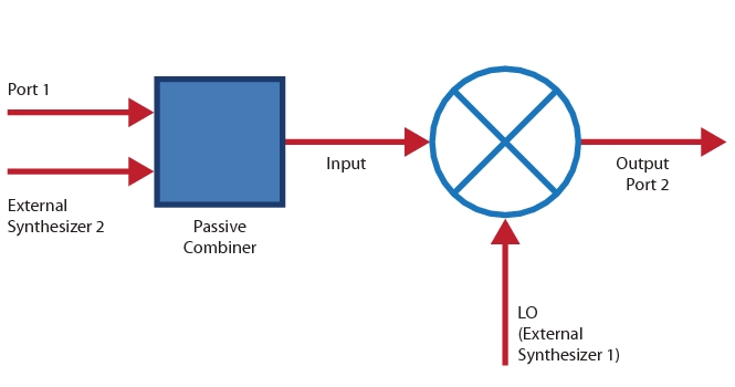
Mixer Setup for IMD Measurement
A simplified setup for mixer IMD is shown here.
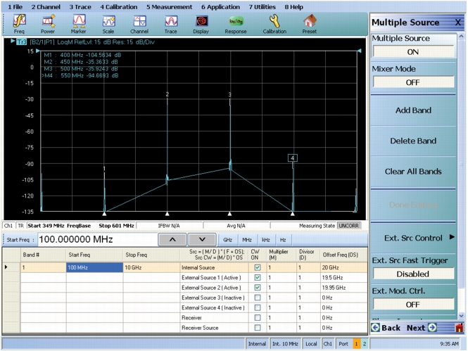
A segmented sweep setup was used in Figure: Example of Multiple Source Setup For CW Mixer IMD Measurement with 11 points (spaced by 200 kHz in this case) around the main tones (a 50 MHz tone offset was chosen), the 3rd order products and the 5th order products. This can optimize measurement time by not measuring frequencies that are not of interest and it allows one to measure quickly when at the main tones (large signals) and in a narrower IFBW when measuring the products (since they may be close to the noise floor). External synthesizer 2 was used to create the 2nd tone and its amplitude was adjusted to make the main tone levels approximately equal although other values could be chosen. In this example, the upper and lower products are not symmetric which may be an indication of bias network interaction within the DUT, compressive behavior in parts of the DUT, or other memory effects.
Example of Multiple Source Setup For CW Mixer IMD Measurement
A multiple source setup for an example CW mixer IMD measurement is shown here.
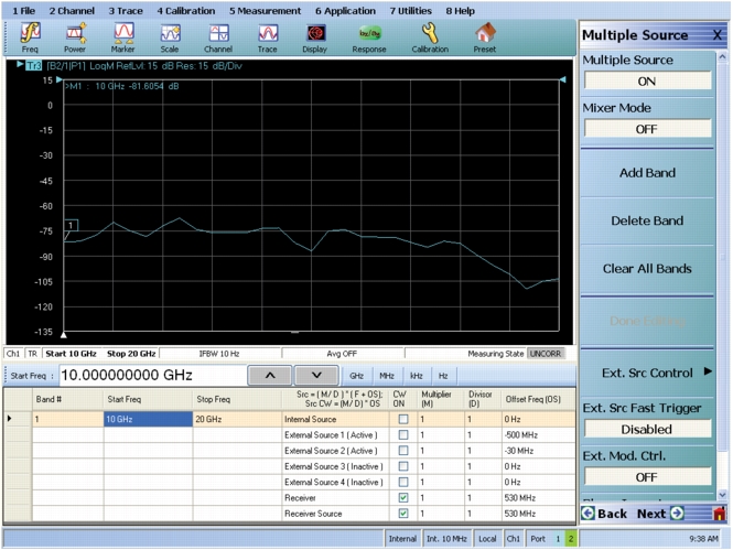
The swept measurement is shown in Figure: Example of Swept Mixer IMD Measurement where the LO is fixed but the two source-like synthesizers are sweeping along with the receiver. In this case the tone offset was chosen to be 30 MHz. The only practical limit (outside of DUT bandwidth) is that very small offsets may incur a noise penalty and the synthesizer noise skirts start to interact. This normally does not happen until below 1 MHz offset depending on the synthesizers being used. The receiver is kept locked onto the upper IMD product in this case. Here just a receiver calibration was used so the readout is the product in absolute power terms (dBm). By doing a sweep with the receiver at a main tone (470 or 500 MHz in this case) and doing a trace(/)memory normalization, one could then measure the product in relative (dBc) terms.
Example of Swept Mixer IMD Measurement
An example swept mixer IMD measurement is shown here.