A common measurement process is to look at harmonics or IMD content at the output of a DUT and the spectrum analysis application can make this very easy visually when the DUT is driven at a single frequency. External sources can be used as the stimulus or the internal source(s) can be employed. Whichever source is used, the harmonic content of that source can limit measureable DUT harmonic content. The internal source harmonics (2nd and 3rd) are generally below -20 to -30 dBc but fractional harmonics may also be present (and can be significant at mm-wave frequencies). These levels can be checked using a thru line measurement or using the reference receivers.

Similarly, source-side IMD products are possible but are generally not an issue except when measuring very low distortion products. More information is contained in IMDView™ (Option 44). For both harmonic and IMD measurements, it is, of course, always important to keep the receiver levels well below the compression point (nominally 0.1 dB compression at 10 dBm but this varies somewhat with frequency, see the Technical Data Sheet for more information).

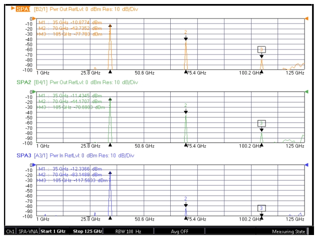
Consider a reasonably complex measurement example using the ME7838 series of broadband/mm-wave systems to make harmonic measurements over an extended frequency range. The DUT in this case was an amplifier with two outputs and both were monitored using two VNA ports and a third port was used as the stimulus source (on a ME7838A4X four port system). The a3/1 (driving port) signal was also monitored to allow visualization of source harmonics. In this particular example, the stimulus was at 35 GHz and receiver calibrations were performed on the two test receivers of interest (b2 and b4) and the sourcing-side reference receiver (a3). The VNA-like sweep mode was used to save measurement time (since we know exactly where we are looking) and a 1 GHz step size was employed at a resolution bandwidth of 100 Hz. Note that in the spectrum analysis setup dialog, the 'Broadband to 125 GHz' selection was chosen for this ME7838A4X system.

Trace 3 (a3/1) in Figure: Example: Harmonic measurement for a two-output DUT. shows the reference (sourcing side) response and one can see the 2nd harmonic is at approximately -71 dBc (3rd harmonic below -100 dBc) and is probably not affecting the measurement. The DUT output harmonics are visible on traces 1 and 2 and one can see the 2nd harmonic is on the order of -33 dBc and the 3rd harmonic is at about -67 dBc. The DUT outputs are reasonably symmetric, but are certainly not at identical levels.

Another spectrum analysis use case is that of Max Hold (and, sometimes, Min Hold) where the instrument monitors a particular frequency range and the largest amplitudes of an external signal are captured across frequency. Examples include capturing the power envelope of a free-sweeping source, trying to quickly gather maximum power output over frequency of a transmitter, identifying the larger transient signals that appear vs. frequency, etc. In this VNA option, this capability is implemented using the Equation Editor and the functions MAXHOLD() and MINHOLD(). The argument for these functions is the trace containing the response variable of interest (e.g., b2/1). The sweep range of the instrument is set to anything that may be of interest for the signal source being analyzed (within the range of the hardware, of course).

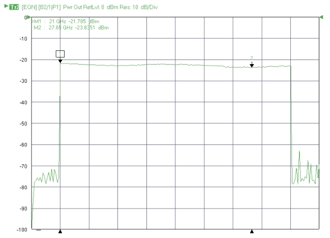
As an example, a free-sweeping source, nominally sweeping over 21-29 GHz, was connected to the VNA port 2. We wished to evaluate its maximum power flatness over this range (the variation at a particular frequency was known to be small). For simplicity, the VNA was set to sweep over 20-30 GHz and Tr2 was set up with the equation editor function MAXHOLD. The result is shown in Figure: The MAXHOLD plot (note the [EQN] annunciator for the equation editor) of the output of a free-sweeping signal source.. One can see the output values had a spread of about 2 dB over the 21-29 GHz range. At the extreme edges of the receiver sweep, one can see the MAXHOLD values of the noise floor. A relatively wide RBW was used for this measurement as the in-band values were of primary interest.

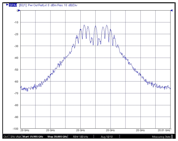
Modulated measurements are also possible but, due to the nature of the image rejection process, modulation bandwidths wider than about 50 MHz will result in some image corruption. A simple FM example is shown in Figure: A wideband (in the sense of modulation index, not actual bandwidth) frequency modulated signal was measured. where the modulation index was 4 leading to the usual Bessel-like sideband dependence. Manual RBW control happened to be used for this measurement and sweep-by-sweep averaging was used in lieu of video bandwidth (VBW) control. The effective filtering bandwidth of sweep-by-sweep averaging is related to sweep time so will end up being sub-kHz for almost all practical setups. As always when measuring a modulated signal, consider the integrated power and power statistics when evaluating the level against the receiver compression point.

Note that the above example was with a very simple stationary signal (in the statistical sense). If a non-stationary modulation is used (i.e., most practical communications traffic) and the symbol rate is rapid compared to the measurement rate, the image rejection will degrade.

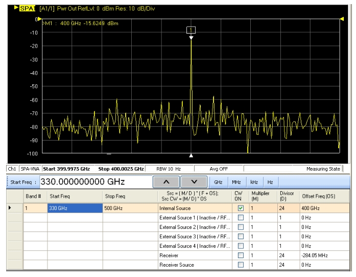
Another example reaches into the higher mm-wave frequencies where 3rd party mm-wave modules may be employed. This requires the direct editing of multiple source control entries (see Multiple Source Control (Option 7)) after entering the spectrum analyzer application. It was desired to look at the spectral characteristics around a 400 GHz signal (locked to the 10 MHz time base of the VectorStar) using mm-wave modules employing a 24 multiplication factor. As shown in Figure: Example: Spectral Content Measurement of a Signal at 400 GHz, the receiver and receiver source equations are set up with a 24 divisor and the receiver offset variable should be set to -(N-1)*12.35 MHz, where N is the divisor. The source was also programmed with its divisor so it could be used for receiver calibration. Note that the multiple source band definition had to be set manually for the module being used. Again, more information on the general setup and use of these modules is available in Multiple Source Control (Option 7).