Although some trace manipulations were alluded to in the previous section, there are considerable trace computation capabilities that warrant further discussion. The simplest of these is TraceMemMath where some operation (addition, subtraction, multiplication or division) is applied between current trace data and that stored in trace memory for that trace. Some points of interest:
• The math is always applied on the basic, linear complex numbers….not on the displayed, formatted numbers.
• Example: The trace is formatted as log mag + phase, the first data point is plotted at 20 dB, 0 degrees and the first memory point is plotted as 40 dB, 90 degrees. Data(/)Memory is selected. This will be computed as (10+j0)/(0+j100)=-j0.1. The result will be displayed as –20 dB, –90 degrees.
• It does not matter if the entire complex value is being presently displayed (e.g., a real-only graph type), the math will be applied to the entire complex number.
• If the user is commonly using log mag graph types, the math may appear counter-intuitive. If one is measuring S21 with a thru line connected, stores data to memory and selects Data(/)Memory, the immediate result is a flat line near 0 dB since one is dividing current data by something very similar (hence close to 1 in linear terms). If one selects Data(–)Memory, the result will be bouncing near the noise floor since now one is plotting the 20*log10(|X–Y|) where X and Y are nearly identical.
• The math is applied after smoothing.
• The math may be applied before or after group delay, depending on the user selection for order of operations (this matters since group delay is computed as a derivative of phase, so if trace match comes first, it acts on phase).
The math is applied before self-normalization (as used in gain compression).
Now that the math is defined, the trace memory behavior needs to be discussed. Historically, Anritsu VNAs had one memory associated with each trace and they were not accessible from other traces or channels. If the number of points is changed, a stored memory will not be available (but will again be available if the number of points is changed back). Trace memory data (formatted or not) can be saved or recalled into that same trace memory location.
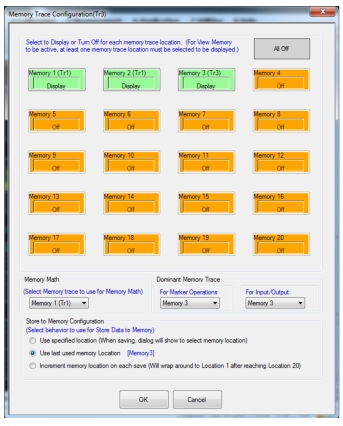
Now there is a more flexible definition where there are 20 trace memories per channel and they can be shared amongst the traces. The point count rules are unchanged. The default behavior is the same as the historic model in that a store operation from trace X will be to memory location X and, by default, TraceMemMath will use memory location X. The control dialog is shown in Figure: Memory Trace Configuration Dialog Box.
Memory Trace Configuration Dialog Box
The matrix in the upper portion of the dialog controls which memories are visible in the current trace (current trace denoted in the title of the dialog) when the display selection is either Memory or Data and Memory. Each box is a toggle button to display or not display the memory and a given button will only be active if something has been stored in that location. The trace where that stored data originally came from will be shown in parentheses (the first two memory locations have data originally from trace 1 and the third location contains data originally from trace 3 in the above example).
The Memory Math pull-down selects which memory will be used for a math operation of the form DataMemMath (discussed previously). The various locations will only be available if something has been stored in that location.
The Store To Memory Configuration section controls what happens when Store Data To Memory is selected. The default is to use the last used location. Thus if this dialog has not been used, it will default to using the location with the same number as the active trace. Another choice is to force a location selection dialog to appear every time data is stored. The final choice is to sequence through all of the memories beginning with the last used location for that trace. This selection is handy when one wants to capture evolutionary data from a DUT (with time, bias conditions, etc.) and it is inconvenient to save data to a discrete file each time. Note that when the 20 locations have been used up with this approach, the oldest stored information will be overwritten and the saving will continue cyclically.
Finally, certain tasks can only deal with one memory per trace so a ‘dominant’ memory can be selected for the active trace. One of these tasks groups are marker operations on memory (searching for targets, etc.). Another task group is saving and recalling of trace memory information (formatted or unformatted). These dominant memory locations default to the same numbered location as the current active trace and can be selected independently for the two task groups.
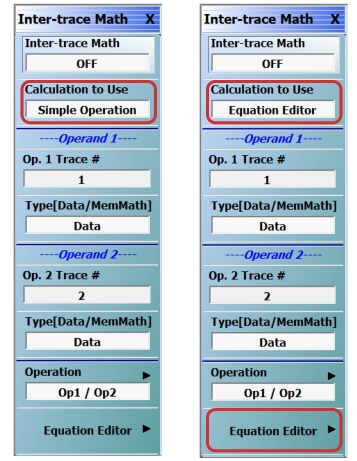
Inter-trace Math
This function allows one to combine measurements from two traces into a result to be plotted in a third trace position. In the Simple Operation mode, the concept is very similar to trace math just discussed, the available operators are the same and the operations again occur on the base, linear complex value. The difference is that the input variables can come from different traces (with completely different S-parameters or user-defined parameters) and can even be based on trace math in that different trace (hence the Type selection in the menu shown in Figure: Inter-trace Math Menu).
Inter-trace Math Menu
Depending on the ‘Calculation To Use’ selection, either a simple (+ - * /) operation set with two arguments is allowed (Simple Operation) or a much more complete set of operations and arguments are possible (Equation Editor).
An example could be someone wanting to measure S21/S12 for a device as a measure of reciprocity (e.g., the device is an isolator). If trace 1 was configured as S21 and trace 2 was configured as S12, then the above settings for the Simple Operation would allow a display of the ratio in real-time. In contrast to basic trace math (where one could measure S21, save it to memory, then change the measurement to S12 and plot DataMemMath) which would be quasi-static, the inter-trace measurement version allows for observing changes during tuning correctly. On a more advanced level, one could normalize each of the input variables using DataMemMath on those traces and then operate on the normalized variables using Inter-trace math (e.g., Tr1/Mem1 + Tr2/Mem2).
Equation Editor
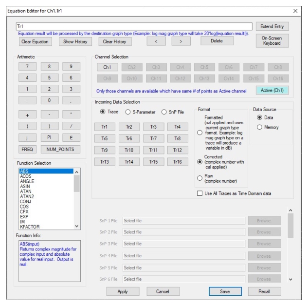
The Equation Editor allows a much more complete set of operations between trace data sets (and S-parameter sets) than does the Simple Operation inter-trace math just described. The main dialog is shown next (see Figure: Equation Editor Dialog—Trace Mode and Figure: Equation Editor Dialog—sNp File Selection Mode) and consists of a selection of functions, input variables (traces and s-parameters in various formats, and sNp file selection) and scalar entry along with some editing tools.
A central concept is that the entire equation is based on complex vectors (which is how trace data and S-parameters come in and what is desired for plotting) of length equal to the number of points. Scalars (real or complex) can be used throughout but, where necessary, will be automatically vectorized (same value at each position in a vector of length equal to the number of points).
Example:
Trace 1 has three points [1+j1, 2+j2, 3+j3]. The equation is Tr1+pi. The result of the calculation will be [(1+pi)+j1, (2+pi)+j2, (3+pi)+j3].
Syntax errors will be flagged if parentheses are not used to resolve precedence problems (e.g., Tr1 * –T2 will not be accepted but Tr1 * (–Tr2) will be).
If the input variable format is selected as Raw or Corrected, the variable will enter the equation as a linear complex number (either with or without calibration applied; note that receiver calibrations are applied to all). If Formatted is selected, the current graph type format will be used so the vector may be purely real. The formatted data can cause considerable confusion (e.g., taking log10 of a variable that is already in dB), but can be useful for some computations (e.g., computing 3rd order intercept in dB from product tone levels in dBm). Note that the graph type used for the equation output will act on the equation result directly (e.g., a logmag graph type will take 20*log10(abs(equation output)) ).
If the time domain checkbox is selected, all traces and parameters will be processed into time domain in the background if they are not already displayed that way. Lowpass Processing will be used if the current frequency list supports it, but otherwise Bandpass Process will be used. Trace time domain parameters will be used, which may be at default if not already configured. It is recommended to configure desired variables in time domain so the results are predictable. See the Measurement—Time Domain (Option 2) chapter of this guide for more information.
Note that trace memory and trace math (discussed earlier in this section) can be used as the incoming variables. Constant π (PI)is available and the 'j' button is used for entering complex scalars. The scientific notation exponent marker 'E' is also available (e.g., 1E9 for 1000000000).
Only single-ended S-parameters are available as direct arguments for the editor. Any mixed-mode S-parameter can, however, be created as a trace variable and used that way as an argument. This is because of the wide variety of underlying port permutations possible with the mixed mode parameters.
Equation Editor Dialog—Trace Mode
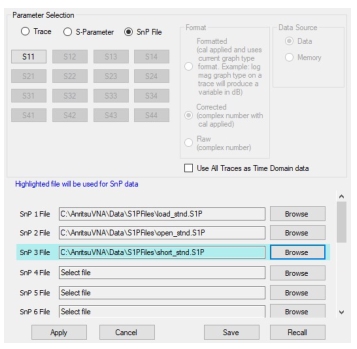
Note that S-parameters from .sNp files may also be used in the equations (see Figure: Equation Editor Dialog—sNp File Selection Mode). Up to 16 files may be used and all S-parameters within a given file (for N up to 4) can be used. Interpolation and flat-line extrapolation will apply when the file frequency range does not match the current frequency range. The data from the files is stored as part of the VNA setup files (and during application shutdown) so the original file location does not need to be maintained. The original file name will continue to appear in the dialog as an aid to remember the nature of the data.
Data (and memory and processed results) from other channels may also be used in the calculation for the active channel. This is particularly useful when data over other sweep ranges is needed (e.g., values of various harmonics for computation of total harmonic distortion). It is required, however, that all channels being used in the equation must have the same number of sweep points so that the vector lengths will be commensurate (and a channel will not be available for variable inclusion if it has a different number of sweep points). The various channels do not have to use the same frequency range, although they commonly will be related (e.g., by a harmonic). Also, the data from the various channels being used in an equation will all be converted to time domain if that checkbox has been selected for the current equation.
Equation Editor Dialog—sNp File Selection Mode
Supported Complex Functions
Following are description of the more complex functions supported (the output of the function is complex unless otherwise noted).
• ABS()—Complex magnitude for complex input and absolute value for real input. Output is real.
• ACOS()—Arccosine; radian output. This will accept complex arguments and uses the standard branch cut.
• ANGLE()—Phase of complex input; radian output. Output is real.
• ASIN()—Arcsine, radian output. This will accept complex arguments and uses the standard branch cut.
• ATAN()—Arctangent, radian output. This will accept complex arguments and uses the standard branch cut.
• ATAN2()—Arctangent with the ability to properly resolve quadrants. The argument is complex and it is internally split into real and imaginary components with sign checking. Radian output
• CONJ()—conjugate
• COS()—Cosine, radian input. Note that this function will accept complex inputs and treat them as such. Commonly one would use this function only with a formatted trace set up for phase and then multiplied by pi/180 to convert to radians.
• CPX(a,b)—Complex equivalent taking 2 real inputs; output is a+jb. If the inputs are complex, the real part of each is taken prior to combination into a new complex variable.
• EXP()—Exponential
• IM()—Imaginary part of a complex input. Output is real.
• MAG()—Magnitude accepting complex input (same as ABS). Output is real.
• MAX()—Maximum value of the MAGNITUDE of the variable selected. (Note that this updates only after a sweep completes so there may be a one sweep delay until the value propagates to a plotted equation). Output is real.
• MAX_HOLD()—Accumulates maximum value of the MAGNITUDE of the argument sweep-to-sweep. The process is reset by clearing the equation or turning inter-trace math off. (Note that this updates only after a sweep completes so there may be a one sweep delay until the value propagates to a plotted equation). Output is real.
• MEAN()—Average value in a complex sense; (note that this updates only after a sweep completes, so there may be a one sweep delay until the value propagates to a plotted equation)
• MEDIAN()—Median value of the MAGNITUDE of the argument; (note that this updates only after a sweep completes, so there may be a one sweep delay until the value propagates to a plotted equation). Output is real.
• MIN()—Minimum value of the MAGNITUDE of the argument …(note that this updates only after a sweep completes, so there may be a one sweep delay until the value propagates to a plotted equation). Output is real.
• MIN_HOLD()—Accumulates maximum value of the MAGNITUDE of the argument sweep-to-sweep. The process is reset by clearing the equation or turning inter-trace math off. (Note that this updates only after a sweep completes, so there may be a one sweep delay until the value propagates to a plotted equation). Output is real.
• MRKX()—Readout of active maker on entered trace, x-value. If no marker is on, a 0 will be returned. If more than one marker is on, the active marker will be used. Output is real. Since this function relies on a trace marker value, the argument can be ONLY a trace and not a function involving a trace.
• MRKY()—Readout of active maker on entered trace, y-value. If no marker is on, a 0 will be returned. If more than one marker is on, the active marker will be used. Since this function relies on a trace marker value, the argument can be ONLY a trace and not a function involving a trace.
• PHASE()—Same as ANGLE but degree output. Output is real.
• POW(z,n)—Raises a complex variable z to the nth power. n is a scalar.
• RE()—Returns real part of a complex input. Output is real.
• REWRAP()—Rewraps phase of a complex variable when range was truncated (often by a power function). The calculation is based on slope of low frequency data.
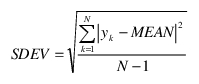
• SDEV()—Standard deviation of input data. This is evaluated only at sweep completion, so there may be a one sweep delay for values to propagate to a displayed equation. This calculation is based on the equation below where N is the number of points. Note that the output is real.
Equation 13‑3.
• SIN()—Sine. Note that this function will accept complex inputs and treat them as such. Commonly one would use this function only with a formatted trace set up for phase and then multiplied by pi/180 to convert to radians.
• SQRT()—Square root; standard branch cut
• SUBSET—(scalar, scalar, vector) returns a subset of the trace/parameter variable that is the third argument. The first two arguments are the point count indices (starting from 0) of the start and stop points of interest.
• TAN()—Tangent. Note that this function will accept complex inputs and treat them as such. Commonly one would use this function only with a formatted trace set up for phase and then multiplied by pi/180 to convert to radians.
• XAXISARRAY()—Generates the vector corresponding to the current sweep variable. Output is real.
Example Using the Equation Editor
Power-added efficiency measurements (PAE) are a simple example of how the equation editor can be used. This measurement makes use of the Analog In ports to measure the DC power consumption of a DUT during a sweep and uses it to compute DUT efficiency so it can also be plotted with other sweep data. Power-added efficiency (PAE) and related metrics are important quantities used in the assessment of amplifiers as well as other devices and subsystems/systems. The efficiency of the use of DC power for RF power generation is critical for the overall performance of many systems and increasingly has a considerable influence on product design. It may be useful to directly measure this quantity on a VNA during other measurements and tools exist to make this feasible in the VectorStar family of instruments. The purpose of this note is to show some of the possible hardware configurations of this in-line analysis as well as how the instrument software can be set up to perform the calculations and display/output the results.
The Method
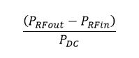
While many definitions exist for PAE, in the end it will be some expression of output RF power relative to input DC power. There may be differences in if gate power dissipation is included or not or at what plane the RF powers are measured, etc. For the purposes of this note, we will use a common definition of:
Equation 13‑4.
Where all powers are expressed in consistent non-logarithmic units (e.g., all W or all mW), the DC power is that fed to the drain or collector terminals (or any single measurable terminal) and the result is expressed as a percentage.
The reader may be familiar with using calibrated wave variables in a VNA to measure RF power: commonly |b2|2 for the 2-port measurement where the DUT output is at port 2, and |a1|2 for the input power. A receiver calibration is required to get an absolute power value for these quantities and the units will normally be mW (and this process absorbs reference impedance terms normally seen).
The DC power measurement process using a VNA may be less familiar but there are two analog input ports on the VectorStar that can be used to measure low frequency quantities synchronized with the sweep. With an appropriate sense resistor, or other current-to-voltage converter, one of these can be used to measure DC current supplied to the DUT. A fixed voltage can be assumed (to compute DC power as I*V) or the second analog input can be used to measure voltage at some relevant node. Note that the two analog inputs multiplex to a single analog-to-digital converter so, if both are used, the sweep will slow down as the system measures both inputs at each sweep point. Thus, if one of the DC parameters (current or voltage) can be assumed constant, it will save some measurement time if that parameter is not actively measured.
Some other important notes about the analog inputs:
• Input impedance: 60K ohms
• Range: –10V to +10V
• Accuracy: a slope and offset calibration is available resulting in a typical accuracy of 2 mV + 2%. Example: for a 1V input, the expected accuracy would be +/- 22mV. The user can refresh this Analog In calibration at any time and is recommended when there are significant temperature changes and low-level signals are being measured.
• Connectors: BNC(F); outer shield is chassis ground (see notes below on sense resistor measurements).
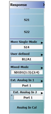
The Analog In measurement is activated by assigning one of the analog in response variables to a trace (instead of, for example, assigning an S-parameter or a wave variable to that trace). These selections are available at the bottom of the response menu as shown in Figure: Response Menu where the response menu in shown where external Analog In signals can be selected for analysis. Note that a driving port must be linked to the analog in variable which ensures that the variable is measured during the desired RF sweep.
Response Menu
The resulting Analog In value generated for plotting is always real so a Real graph type is recommended for viewing. A Lin Mag graph type is also possible if polarity is not of interest. Imaginary graph types will always yield zeros and phase graph types will produce 0 degrees or 180 degrees. The real (or linear magnitude) graph type marker readouts are labeled in Units (U) which should be interpreted as Volts (V) for Analog In.
One note on measuring current: since the analog in inputs have a ground reference, one cannot usually measure the voltage across a sense resistor directly using one input. Instead, one can measure voltages at both ends of the sense resistor, using the two inputs, and get both voltage and current.
For certain measurement setups with high bias network impedances, the 60kohm input impedance may load the circuit. In these cases, a buffer amplifier or other transforming structure may be needed.
The Calculations
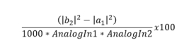
The user may export data of |b2|, |a1| and the desired analog in variables and compute PAE themselves (where those variable names assume a 2-port setup where the DUT input is port 1 and the output is port 2). If one assumes current was measured with a current-to-voltage converter with a transimpedance of one ohm (using AnalogIn1) and the voltage was measured directly on AnalogIn2, the PAE would be given by the following if needed receiver calibrations are in place:
Equation 13‑5.
Here the numerator will be reporting in mW (and the wave variables should be exported in a Lin Mag format or converted to that). Since the AnalogIn1 will represent current in Amps by virtue of the sense resistor, a factor of 1000 is needed to also get the denominator into mW. The final factor of one hundred is to convert PAE into a percentage.
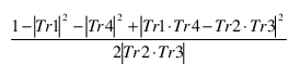
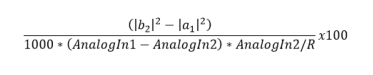
If, instead, a sense resistor (of value R ohms) was used, the DUT-side voltage was measured on AnalogIn2, and the supply-side voltage measured on AnalogIn1, then one would calculate:
Equation 13‑6.
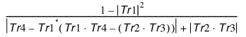
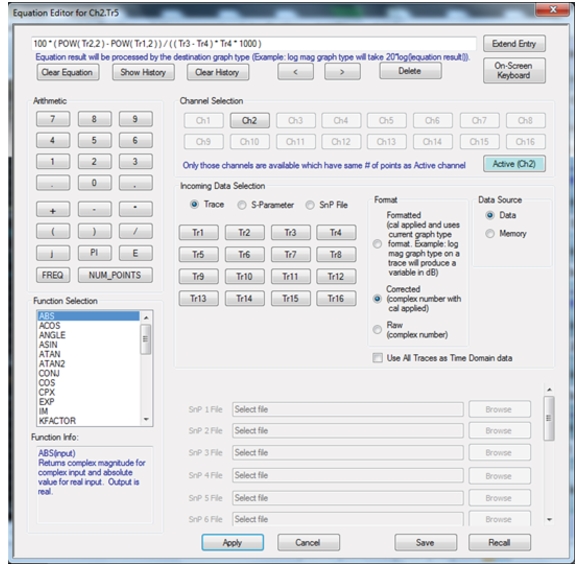
The Equation editor in VectorStar can also be used to implement this computation and plot the result in an additional trace. That formulation of the previous equation (assuming Tr1 is a1, Tr2 is b2, Tr3 is AnalogIn1, Tr4 is AnalogIn2, and the sense resistor is one ohm) is shown in Figure: Equation Editor where the Equation Editor is setup for computing PAE using a sense resistor is shown here.
Equation Editor
Note that formatted variables were used for the equation which means the graph types for those traces need to be set correctly (Lin Mag for the wave variables and Real or Linear Magnitude for the Analog In variables). More information on using the Equation Editor is available in Trace Math, Inter-trace Math, and Equation Editor.
Example
An E-band LNA was the test device (and its PAE was expected to be very low) and it was of interest to see how PAE varied with RF drive power at 89 GHz. This measurement made use an ME7838D broadband system to get the frequency coverage, but the ideas here apply for any frequency range and any VectorStar family model.
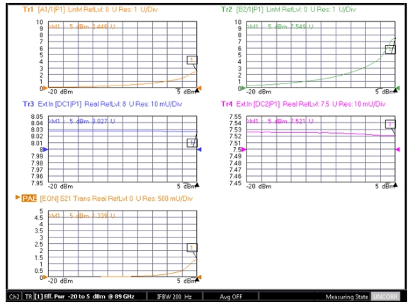
Receiver calibrations were performed for a1 and b2 receivers as they will represent input RF power and output RF power, respectively. These measurements were assigned to traces 1 and 2. A 1 ohm sense resistor was used, and the DUT-side voltage was connected to AnalogIn2. The supply-side voltage was connected to AnalogIn1. The RF power was swept from –20 to +5 dBm. The graph types and response variables were assigned as discussed in the previous section and the measurements are shown below. The equation editor output was assigned to the trace at the bottom of Figure: PAE Measurement (changed to have a trace name of PAE). About 0.5V is dropping across the sense resistor so DC power dissipation is about (0.5V/1ohm)*7.5V=3.75W. Given the <10mW max power output of the device, PAE will be low and indeed it is (at little over 1% at high drive). The result of an example PAE measurement of an E-band amplifier in a power sweep is shown in Figure: PAE Measurement (in the bottom trace, expressed as a percentage)..
PAE Measurement
One can see that the DC power consumption is increasingly slightly at higher drive levels (the DUT-side voltage on the sense resistor in Tr4 is dropping so current draw is increasing) but this is outweighed by the increase in RF output power so the efficiency increases.
A Real graph type was used for the equation editor output which is a desirable choice given the calculation and the value should be read as a percentage because of the 100x factor in the equation.