A traditional frequency sweep is based on a start frequency, a stop frequency, and a number of points (or, alternatively, substitute center/span for start/stop). The number of points is not confined to certain preset values. The minimum number is two (otherwise use CW mode) and the maximum number is usually 25,000.

A mode allowing 100,000 points is also available, but operation is limited to a single channel.

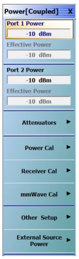
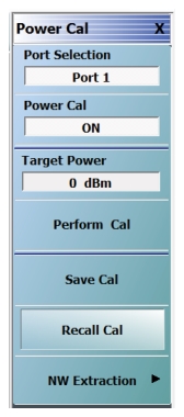
Power entry while in frequency sweep mode is accomplished through the MAIN POWER menu and the POWER CAL menu for frequency sweep, as shown in Figure: Main POWER Menu—Port 1 and Port 2 Coupled—Attenuators Installed and Figure: POWER CAL Menu.

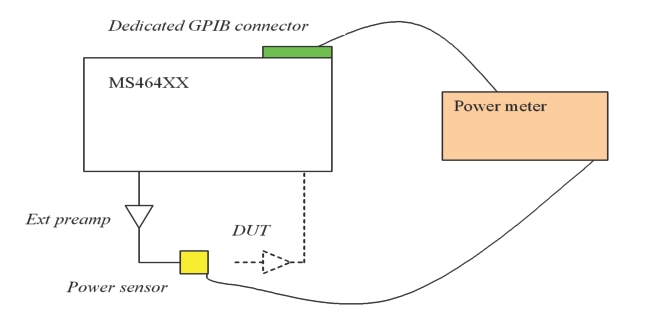
The objective of the power cal is to improve the accuracy of the power delivered to the DUT beyond that provided by the factory ALC calibration (0.1 dB vs. on the order of 1 dB). This is particularly useful if a preamplifier or other network is needed between the test port and the DUT. The exact loss/gain of that network over frequency can be corrected for with reasonable precision. A common setup for executing this calibration is shown in Figure: Port 1 Power Calibration Example Setup.

The relationship between the power entry fields and the Target Power field of the power calibration is important. First a few definitions:

The normal procedure is to enter the desired power at the user reference plane (where the power sensor will be connected for the power calibration). If the gain/loss between the VNA port and the user reference plane is small, the ALC entry field can be set to the same value as the Target Power. If the gain/loss is significant, the ALC field should be offset by an estimate of that gain/loss (ALC entry field should be higher if it is a loss, and lower if it is a gain). This offset need not be extremely accurate; it serves to inform the system of where roughly to set the internal sources in order to achieve the desired user reference plane power. After the power calibration is completed, the Effective power field will match the Target power. If the ALC entry field is later changed (from the value at the time of the calibration), the Effective power field will also change to reflect an estimate of the new user reference plane power. This new value is only an estimate since the calibration was not performed at that power level and the accuracy will decrease as the change from the calibrated level increases.

Target power is –20 dBm and there is about 8 dB of loss from the VNA port to the desired reference plane.

Note that the source attenuator settings (if Option 61 or 62 is installed) will be reflected in the Effective Power value, even if no power calibration is applied.

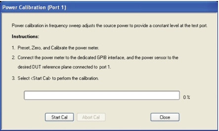
Since the power cal performs the calibration at every point, this calibration can be time-consuming (particularly if a slower thermal power sensor is being used). One should exercise some restraint when selecting the number of power points if this time delay will be an issue. Details of power meter connection and setup are covered in the Operation Manual, but one should ensure that the power meter GPIB address matches that shown on the MS464xB Series VNA GPIB menu system and that the dedicated GPIB connector on the VNA is used. The dialog that appears when executing this calibration is shown in Figure: POWER CALIBRATION (PORT 1) Dialog Box.

Many possible power meters/sensors can be used with the MS464xB VNA and these choices proliferate with the broadband and millimeter wave versions (see Broadband/mmWave Measurements (Option 7, Option 8x) of this guide) so some guidance may be helpful:

When not in broadband mode, the user will have the option to select a USB sensor if one is detected. If not, the system will first scan for the Ext. Power Meter address and will use that meter if found and the reported frequency ranges match (note that 437B emulating meters do not report a frequency range so the system will use them regardless). If such a meter is not found, it will next search for the Broadband meter. If that is also not found, the calibration will terminate with an error.

In broadband modes, there are many more choices and the system will switch between sensors/meters to cover the desired range. This is perhaps illustrated best with a series of examples and those are in the chart shown in Table: Power Sensor Selection Guide (1 of 2). The system will start from the left of the chart and use the first option (or combination) that is available. Many of the sweep ranges in the chart are only possible with the ME7838x broadband systems (see Broadband/mmWave Measurements (Option 7, Option 8x) of this guide for more information).

Whatever the basic power meter accuracy is will be transferred to the VNA within about 0.1 dB (convergence criteria is normally 0.07 dB, this limit loosens for frequencies above 70 GHz) for short periods of time. That correlation can drift as temperatures change, connection repeatability, etc. The basic accuracy of the power meter is outside the scope of this guide (consult the documentation for the meter/sensor in question) but includes terms such as linearity, mismatch, basic power factor correction, offsets, and other items.

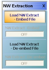
An additional function possible with power calibrations is embedding or de-embedding where an existing power calibration is modified by the S-parameters in a .s2p file to reflect a network that was added after the power calibration (embedding) or removed after calibration (de-embedding). These functions are placed on a submenu labeled NW extraction (short for network extraction, this refers to the calibration options submenu where the .s2p file is often generated). They are accessed by selecting Power | Power Cal | NW Extraction. Figure: NW EXTRACTION Menu shows the NW Extraction menu, which is enabled only if a power cal exists.

This menu enables one to load files separately for embedding and de-embedding. Note that the files are separate for port 1 and port 2 power calibrations. Also note that only the S21 parameter is used in the adjustment of the power calibration (and, of course, only the magnitude). Interpolation and extrapolation are used if the frequency lists of the .s2p file and that of the power calibration do not match. A warning dialog will appear if extrapolation will be used.

If the network loaded is lossy and is being embedded (e.g., the power calibration is performed coaxially and then the reference plane is connected to a wafer probe and the desired reference plane is at the probe tip), the power delivered by the source will increase by the amount of the loss. Similarly, if such a lossy network is de-embedded (e.g., an adapter was used to facilitate the calibration but is then removed for the measurement), the power delivered by the source will decrease by the amount of the loss.

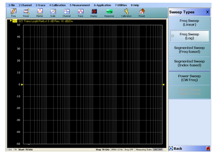
All of the above discussion applies to both linear and log versions of swept frequency. In log sweep, the frequency list is calculated using a constant ratio step as opposed to a constant step size in linear frequency sweep. Also, the graticule for rectilinear plots while in log sweep will change to reflect that modified frequency list. An example is shown in Figure: Example Graticule for the Log Sweep Type. Integral numbers of decades of lines will always be used.