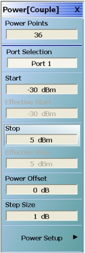
A power sweep is valuable for making gain compression and other power-dependent semi-linear measurements. The frequency is set at a single CW value and the power range is specified in a way analogous to frequency sweeps as suggested by Figure: Main Power Sweep Menu—POWER [COUPLE] Menu.
Main Power Sweep Menu—POWER [COUPLE] Menu
Sweep Type set to Power Sweep (CW Freq)
As with the regular power control in frequency sweep, the power at the two ports may be coupled or uncoupled. This feature takes on new importance in power sweep in that the two ports may drive with completely different power ramps. The number of points in these two power sweeps must, however, be the same. As with all sweep types, different attenuator settings in different channels is not permitted to avoid potential attenuator damage in fast sweeping scenarios.
Power offset is an important entry for cases when an external preamplifier, large pad, or other network may be in use between the port and the DUT plane. By entering a value here to approximate the net gain of the external networks, the effective power fields will be updated accordingly and any power calibrations performed will be more efficient. Note that source-side attenuator settings are also reflected in the effective power fields.
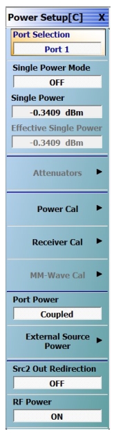
Some of the more detailed controls are on the power setup level of the power menu located on the POWER SETUP menu (see Figure: Second Level Power Sweep Setup Menu—POWER SETUP [C] Menu). The coupling control and port selection (when uncoupled, duplicate of first level) is located here as is the single power selection items. This entry allows one to put the system in constant power (and constant frequency) and is often used for making DUT adjustments prior to full power sweep measurements. The receiver cal and external source power submenus are covered in other sections of this measurement guide (Receiver Calibration and Multiple Source control respectively).
Second Level Power Sweep Setup Menu—POWER SETUP [C] Menu
The Src2 Out Redirection pertains to Option 32 (a combiner option available in dual source systems) where the source 2 signal can be switched to combine into the source 1/port 1 signal path. This switch can be activated here when using manual multiple source measurements but is overridden in the IMD measurement (see IMDView™ (Option 44)).
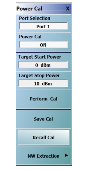
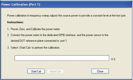
The power calibration while in power sweep mode allows an accuracy enhancement of the power levels delivered to the DUT. A power sensor will be connected to the port selected and then at each power point in the power sweep, the system will adjust the control loops to deliver that power to within 0.1 dB. The Power Calibration menu is shown in Figure: POWER CAL Menu and the dialog executing the calibration is shown in Figure: POWER CALIBRATION Dialog Box. Note that the Target power range will want to maintain the span of the power menu entries (e.g., if the main start power is –10 dBm and the main stop power is 5 dBm, the target power spread should normally be 15 dB). This comes from an assumption that the target difference would be due to a loss or gain offset rather than some heavily compressing medium.
POWER CAL Menu
POWER CALIBRATION Dialog Box
Gain Compression
Although not a sweep type by itself, gain compression is often thought of as the main application of power sweep. As such, a trace-based utility is provided to simplify the gain compression measurement.
The objective is to provide a marker-like function for quickly finding the X-dB compression point of an amplifier or other DUT. While this is typically performed on S21, it is allowed on any ratioed parameter so that, for example, match deviations can be quantified during compression. The gain compression function is trace-based, unlike the sweep type, so it can be invoked on some traces (S21 for example) and not on others (b2/1 to monitor output power for example).
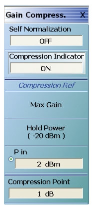
The main gain compression menu (located under Display while in power sweep) is shown in Figure: GAIN COMPRESS. (GAIN COMPRESSION) Menu—Power Sweep CW Set. The second button toggles on and off the indicator for the active trace (the indicator is denoted by a “C” on screen and will be located at the desired compression point. The top button activates continuous normalization of the trace to the value of the first point in the power sweep. This allows for easier visualization of the compression process but is not necessarily needed for the measurement.
GAIN COMPRESS. (GAIN COMPRESSION) Menu—Power Sweep CW Set
Note
The Hold Power value is read-only and comes from the HOLD menu.
The middle three buttons determine how the compression point is to be measured. That is, the X-dB compression marks a decay of X dB from what value? Commonly, this is done from a low power level which is often the hold-state power (see the hold functions menu under Sweep Setup). The reference can also be set to the maximum output power point and this may be useful in cases of gain expansion. Finally, the reference may be set to the point corresponding to an arbitrary, entered input power value.
The compression point can be entered separately and common values are 1 dB and 0.1 dB. Note that this value is allowed to be negative so certain levels of gain expansion can be sensed.
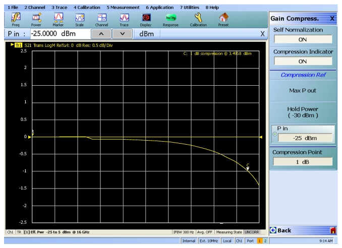
An example measurement showing these features is illustrated in Figure: Gain Compression Example. The input power corresponding to the compression point is readout in the upper right corner of the screen. The compression indicator “C” picks out the 1 dB compression point at an input power of ~3.5 dBm. Note that if Max Gain is selected as the gain reference, the location of the ‘R’ reference marker will move from sweep to sweep as a new maximum point is identified each time. If the data is noisy (e.g., very wide IFBW, very low input power or output power, etc.), the gain reference can change significantly from sweep to sweep and hence the compression point determined may be more variable.
Gain Compression Example
The steps that might be taken in executing the above measurement:
1. Set the CW frequency (16 GHz in this case) and the power sweep parameters (–25 to +5 dBm with 61 power points), A higher density of power points will help with accuracy on the compression point (so the system has less interpolation to do) at the expense of longer measurement time and longer power calibration time (if performed). Select the IFBW (300 Hz in this case) for the desired trace noise level.
2. Perform a power calibration if desired. The factory ALC cal accuracy may be adequate in some applications (generally better than 1 dB at microwave frequencies) but the user power calibrations can improve on this. See earlier comments in this chapter on user power calibrations for more information. Note that with thermal sensors, the calibration time per power point could be 5–10 seconds.
3. Perform an RF calibration if desired. This was not done in this example since the input compression point only was of interest and not the absolute gain. A one-direction transmission frequency response calibration may be all that is needed if absolute gain data is required (does not include match correction but is often adequate).
4. Set up the gain compression parameters. In this case, self-normalization was used to center the result near 0 dB (bases on the 1st point and renormalizes every sweep so it may appear to be jumping if the data is noisy). The 1 dB compression point is of interest (that is the default value) and the compression point was to be referenced to the gain at –25 dBm input so 'Pin' was selected as the reference.
5. Turn on the compression indicator and observe the result.