This specialty sweep type is a hybrid of the power sweep and linear frequency sweep types discussed earlier. The application is used to evaluate compression points across multiple frequencies without having to setup power sweeps individually at each frequency. The nomenclature and the meaning of the displays require some interpretation different from other measurements. In some contexts, this sweep mode is called Multiple Frequency Gain Compression (MFGC).
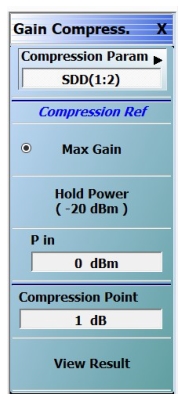
When in this sweep type, the gain compression menu will be available as it is with CW power sweep, but compression determination will always be on and there is no self-normalization. Most of the items are the same as in the single frequency gain compression (CW power sweep), except for the first menu item, as shown in Figure: GAIN COMPRESSION Setup Menu for Power Sweep (Swept Frequency). As with CW power sweep, these selection are all per-trace. This may require some attention as parameters within the channel may be being evaluated at wildly different compression points depending on the setup.
GAIN COMPRESSION Setup Menu for Power Sweep (Swept Frequency)
The compression parameter (Figure: COMP. PARAM (COMPRESSION PARAMETER) Menu), which must be a ratioed S-parameter, is the variable that is used to find the compression point (S21 is usually used for this role).
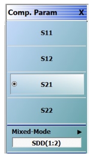
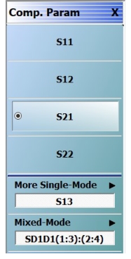
COMP. PARAM (COMPRESSION PARAMETER) Menu
2-Port VNA
4-Port VNA
Note that the compression will be based on an S-parameter and cannot be user-defined. Mixed-mode parameters can be selected as the compression variable and this is useful, for example, with differential amplifiers. If an incomplete calibration is in place, the system will make the required sweeps to compute the selected parameter but, of course, any displayed parameters may have reduced/destroyed accuracy if the calibration does not match the port configuration.
The compression parameter is a per-trace selection; that is, every displayed response parameter can be referenced to compression of a different S-parameter. Commonly S21 will be used for the compression parameter in all cases (on two port systems) but the flexibility is available.
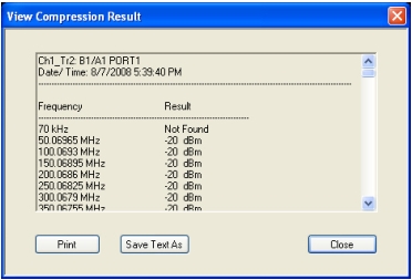
The desired plot variables, which are set up in the usual way with trace and response menus, are then evaluated at the power producing the indicated compression level in the compression parameter. The “view result” button will display (vs. frequency) the active trace parameter at which the desired compression occurred. This display will be in tabular form in a separate dialog (Figure: VIEW COMPRESSION RESULT Dialog Box).
VIEW COMPRESSION RESULT Dialog Box
The dialog shows the value of the active trace parameter at the desired compression point. If the active trace has a two graph display (e.g., log magnitude and phase), there will be a third column added.
Power-Sweep Swept Frequency Example
To help understand these concepts, consider an example. We have an amplifier connected in the usual forward direction (S21 > 0 dB) and we wish to know the output power and the input match when at the 1 dB gain compression point at a few frequencies. Assume that sufficient attenuation is employed to prevent VNA compression and that all needed calibrations have been performed.
• At 1 GHz:
• S21
• = 10 dB at –10 dBm input (low power) and
• = 9 dB at +1 dBm input
• b2/1 (output power)
• = 0 dBm for –10 dBm input and
• = 10 dBm at +1 dBm input
• S11
• = –15 dB at –10 dBm input and
• = –17 dB at +1 dBm input
• At 2 GHz:
• S21
• = 12 dB at –10 dBm input (low power) and
• = 11 dB at +3 dBm input
• b2/1 (output power)
• = 2 dBm for –10 dBm input and
• = 14 dBm at +3 dBm input
• S11
• = –17 dB at –10 dBm input and
• = –18 dB at +3 dBm input
• At 3 GHz:
• S21
• = 7 dB at –10 dBm input (low power) and
• = 6 dB at –1 dBm input
• b2/1 (output power)
• = –3 dBm for –10 dBm input and
• = 5 dBm at –1 dBm input
• S11
• = –10 dB at –10 dBm input and
• = –8 dB at –1 dBm input
The compression points based on the compression parameter of S21 (input power referred) are as follows:
• 1 GHz: +1 dBm
• 2 GHz: +3 dBm
• 3 GHz: –1 dBm
Since output power and input match at 1 dB compression are of interest, one would select b2/1 and S11 as the display parameters. In this sweep type, those parameters will be evaluated at the above power levels established by the compression measurement. A plot of |b2/1| would then show:
• 1 GHz: 10 dBm
• 2 GHz: 14 dBm
• 3 GHz: 5 dBm (assuming a power out graph type is being used and a receiver cal is in place)
A plot of |S11| would show:
• 1 GHz: –17 dB
• 2 GHz: –18 dB
• 3 GHz: –8 dB (assuming a log magnitude graph type)
Any of the normal S-parameters or user-defined parameters can be selected as the display variables (just as in any other sweep type). Those most commonly used are the S-parameters (to represent amplifier quasi-small-signal behavior at the point of compression), an un-ratioed parameter to represent output power at compression (often |b2/1|), and an un-ratioed parameter to represent input power at compression (often |a1/1|). Again, a receiver calibration is required for the representation of absolute power (input or output) and this is discussed in detail in another chapter of this measurement guide.
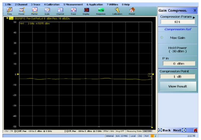
The plot resulting from an example measurement is shown in Figure: Example Plot from Power Sweep with Swept Frequency. Here the frequency sweep range was 1–2 GHz while the power sweep range (at each frequency point) was –10 to +5 dBm. The display parameter is output power (|b2/1|) while the compression parameter is S21.
Example Plot from Power Sweep with Swept Frequency
The detailed series of steps that might be used to arrive at the above measurement could follow this script:
1. Select the frequency and power ranges and number of points for each range. (1 GHz to 2 GHz with 51 points, –10 to 5 dBm with 16 points). The power sweep range should, of course, include the anticipated compression point. It may be tempting to use more points, but power calibration time and measurement time will vary as (frequency points)*(power points). As stated earlier, the maximum number of frequency points is 401. Select an appropriate IFBW based on trace noise needs (1 kHz in this case).
2. Perform a power calibration if desired. The factory ALC calibration accuracy may be adequate (<1 dB generally at microwave frequencies) but if not, or if there is a lossy network between the test port and the DUT plane, a user power calibration may be useful. See earlier comments in this chapter on power calibrations. Note that with thermal power sensors or low power levels, the power calibration can take several seconds per point and there are (frequency points)*(power points) points to consider. Interpolation and extrapolation will be used if the ranges are changed after calibration and generally these are smoothly varying functions. Note that a MFGC power calibration can be used in other sweep modes.
3. Perform a receiver calibration if needed. This is important for the current example as we wish to measure output power at 1 dB compression (via b2/1). A thru connection is all that is needed and the calibration is automatically performed at the ‘single power’ value (not across power; the receiver linearity is relied upon for other levels and is better than 0.05 dB except near receiver compression or the noise floor). Interpolation and extrapolation will be used if the frequency range is changed after cal.
4. Perform an S-parameter calibration if needed. This may be important if gain or mismatch at compression is needed and any of the calibration choices are available. If only gain is needed, a one-direction transmission frequency response calibration may be adequate.
5. Set up the gain compression configuration for each trace. In this case the compression parameter is S21 and the reference is max gain. Note that this reference definition is not universally used and can result in surprising values if the DUT has significant gain expansion or other mid-range distortions.
6. Observe the results and view tabular values with the View Result button if desired.
Some points of note:
• Frequency range is setup using the normal frequency menu. The only constraint is that a maximum of 401 frequency points can be used.
• The power sweep range is setup as with CW power sweep. The usual limits on power points apply.
• If one wants to look at the actual gain compression curve (|S21| vs. power for example), set up a 2nd channel, since power sweep (CW) and power sweep (swept) cannot be combined in the same channel.
• S-parameter calibrations are basically handled as in linear frequency sweep. If performed while in this sweep type, they will be conducted at the start power. The same error coefficients will be applied at all power levels. If the calibration was performed in linear frequency sweep, the point count will be coerced in this sweep type to get under the 401 point limit (interpolation will be used if it is active).
• Receiver calibrations are normally required for accurate plots of output power and can be performed in this sweep type or in other sweep types as long as the appropriate frequency range is covered.
• As discussed previously, receiver calibrations fully use interpolation and extrapolation. Distortions can occur at bandswitch frequencies (2.5, 5, 10, 20, 38, and 40 GHz for base VNAs plus 30, 54, 80, 110, 120, 130, 153 and 170 GHz for some ME7838X systems) if interpolation is used and point density is not high. At very low frequencies (<30 MHz), additional transition frequencies occur. When in doubt, one can redo the receiver calibration over the desired frequency list.
• When in this mode, receiver calibrations are performed at the 'single power' power level. Normally, this should be relatively high so as to minimize trace noise but can be any value the system can achieve.
• Power calibrations are also interpolated and extrapolated. Similar bandswitch frequencies play a role but the effects are usually less dramatic than for receiver calibrations (except at mm-wave frequencies >100 GHz).
• Mixer MFGC can be performed using the same steps if a reference mixer is employed (see Mixer Setup and Measurement of this guide for more information; normally such a mixer is placed in the reference loop of the VNA and shares the LO with the DUT). Generally, the reference mixer input is well-padded or is otherwise more linear than the DUT so allow for more unambiguous measurements.