The reader will have noted another submenu in the response category that describes mixed-mode parameters. One is likely familiar with the concept of a differential amplifier and the general concepts of differential and common-mode signals [2] as suggested by Figure: Characterizing Differentially Driven Components. It is clear that it may be useful to represent S-parameter data in a form corresponding to differential drive/reception (and similarly for common-mode). Such a formulation has been developed in the past (e.g., [1]-[4]). The purpose of this section is to describe and define this representation, provide some hints on data interpretation along with explaining how to setup the desired responses.
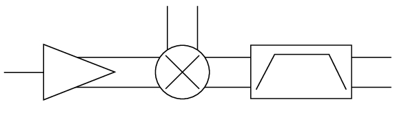
Characterizing Differentially Driven Components
A portion of a common communications circuit is shown here where a number of components are driven differentially. It is of obvious interest to characterize these parts in terms of differential and common mode signals.
The concept here is one of a pair of ports being driven at a time, either in-phase (common mode drive) or 180 degrees out of phase (differential drive). Similarly, we are interested in the received signal in a port pair context: what is the common-mode (in-phase) signal received and what is the differential signal received. In contrast to the single-ended drive and single-ended receive types of parameters are conventionally used, these parameters represent a transformation of the data.
This combined signal drive concept can also be explained pictorially. Each pair (either 1-2 or 3-4) can be driven either in phase (common mode drive) or 180 degrees out of phase (differential drive). For the transformation, it is convenient to group together single ended ports 1 and 2 together as the new Port 1 (which can be driven differentially, common-mode, or some combination). Similarly, single ended Ports 3 and 4 will be grouped as the new Port 2 (same idea: differential, common-mode, or combination). Thus the new basis is to think of a port pair as being driven in phase or 180 degrees out of phase (instead of thinking of each port of the pair being driven individually). The new input and output bases are illustrated below (Figure: Analyzing Mixed-Mode S-Parameters). The reader may recognize this as a simple shift in basis, which can be thought of as a 45 degree rotation.
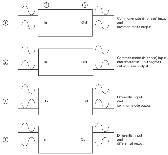
Analyzing Mixed-Mode S-Parameters
The new basis for analyzing mixed-mode S-parameters are shown here. With the physical ports considered as pairs, one can analyze in terms of common-mode and differential drive and common-mode and differential output.
1. Common-mode (in phase) input and common-mode output.
2. Common-mode (in phase) input and differential (180 degrees out-of-phase) output.
3. Differential input and common-mode output.
4. Differential input and differential output.
5. Input Side (at left).
6. Output Side (at right)
A common question is whether these ports need to be driven with pure differential and common-mode signals or whether the same result can be achieved by mathematical superposition of single-ended signals. With certain assumptions on linearity, the answer is yes and the derivation will be presented next. The only practical requirement is that the bulk of any strong non-linearity be after the first differential stage or that there is reasonable common-mode to differential isolation (e.g., [5]-[6]) which is true for many devices even when gain compression is being measured.
The next step is to construct S-parameters for this type of input/output. The possible incident waveforms can be deduced from Figure: Analyzing Mixed-Mode S-Parameters above:
• differential on the new Port 1
• common-mode on Port 1
• differential on Port 2
• common-mode on Port 2
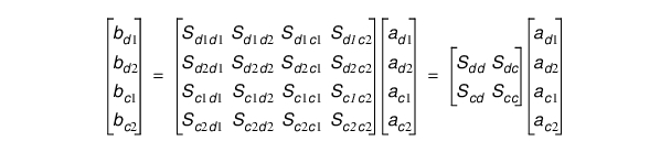
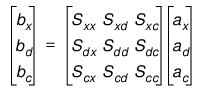
The output waves will have the same structure, which leads to the S-parameter matrix structure depicted in Eq. 24‑2.
Equation 24‑2.
Here the four S blocks in the square matrix to the right are actually submatrices [2]. Sdd corresponds to the four purely differential S-parameters while Scc corresponds to the four purely common-mode parameters. The other two quadrants cover the mode-conversion terms. These are expanded in the center part of Eq. 24‑2. The matrix equation can be interpreted as expressing an output wave bi in terms of the four possible input waves ad1, ad2, ac1, and ac2. An example of one of these sub-equations is shown below.
Equation 24‑3.
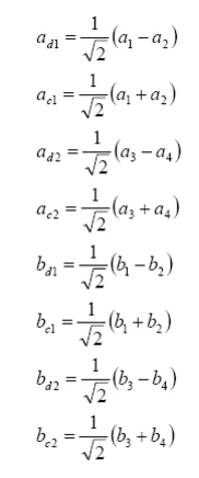
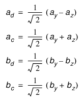
It is straightforward to write the relationships between the single-ended incident and reflected waves and the new balanced versions. To simplify the presentation, the next set of equations will assume port pair 1 is composed of physical ports 1 and 2 while port pair 2 is composed of physical ports 3 and 4. We will show a means of generalizing this construction later. The difference and sum choices are obvious for differential and common-mode waves, respectively, and all else that is needed is a normalization factor to keep power levels equivalent.
Equation 24‑4.
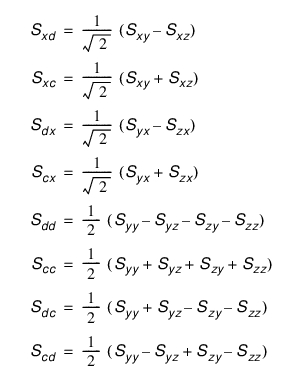
This linear combination of single-ended wave functions makes the transformation particularly transparent. One can define a simple transformation matrix to operate on single ended S-parameters to produce the mixed-mode S-parameters that are shown below. The parameters are grouped by the quadrants labeled in Eq. 24‑2.
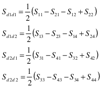
The differential-to-differential terms:
Equation 24‑5.
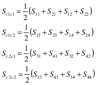
The common mode-to-common mode terms:
Equation 24‑6.
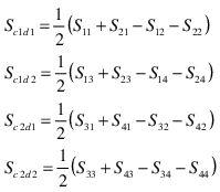
The common mode-to-differential terms:
Equation 24‑7.
and the differential-to-common mode terms:
Equation 24‑8.
The simple linear relationship between the parameters should be evident. Just to reinforce the interpretation of these parameters: Sd2d1 is the differential output from composite Port 2 (the old Ports 3 and 4) ratioed against a differential drive into composite port 1 (the old Ports 1 and 2). Similarly Sc2c2 would be the common-mode reflection off of composite Port 2 ratioed against the common-mode signal applied to composite Port 2.
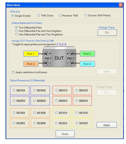
Aside from selecting among the 16 parameters described above, there is also the matter of defining the port pairs. This is accomplished in the middle part of the dialog and note that there is a polarity sense assigned to the pairing (determines the sign of the differential signals). When displaying the parameters, this port assignment must also be conveyed and is done with the following symbolism:
• (A:B):(C:D) (where A, B, C, and D are unique port numbers from {1,2,3,4})
Here, the first port pair is A-B (with A assigned the positive polarity) and the second port pair is C-D (with C assigned the positive polarity).
For example:
• (1:2):(3:4) The first port pair is measured from 1 to 2 and the second port pair is measured from 3 to 4.
• (1:2):(4:3) The first port pair is measured from 1 to 2 and the second port pair is measured from 4 to 3.
MIXED MODE Two Differential Pairs Dialog Box
The dialog for selecting mixed-mode parameters, configured for two differential pairs, is shown here. The instrument defaults to the SD1D1 response.
The 3-port version of these mixed-mode parameters is a straightforward simplification. Port X will remain single ended while ports Y and Z will form a balanced port pair. Following the analysis path from before:
Equation 24‑9.
Equation 24‑10.
Equation 24‑11.
In Equation Group 11 (Eq. 24‑11), the subscript x remains since that port is defined solely as a single-ended port.
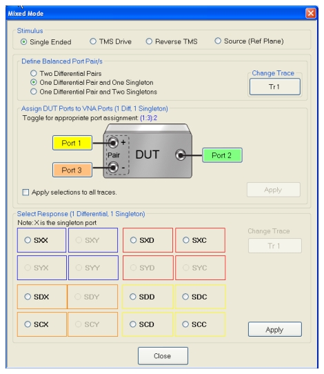
The three port configuration is termed a differential pair and a singleton and the dialog for selecting this type of parameter is shown in Figure: MIXED MODE One Differential Pair and One Singleton Dialog Box. Note that one can define this parameter class even if a 4-port calibration is applied; it is a matter of port assignment. As with the dual differential case, the ports must be assigned with polarity in mind.
MIXED MODE One Differential Pair and One Singleton Dialog Box
For the situation in the figure above (Figure: MIXED MODE One Differential Pair and One Singleton Dialog Box), there will be a different annotation on the graph legends to denote how the ports are configured but it is similar to the two-differential-pair format discussed earlier. (1:2):3 denotes that the differential pair is measured from Port 1 to Port 3 and Port 2 is the singleton.
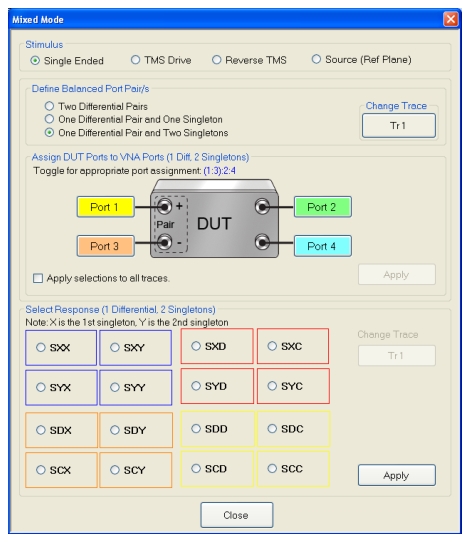
Certain 4-port devices are configured as one differential pair plus two single-ended ports. The parameters can then be configured in a one differential pair and two singleton format. The mixed mode definitions are identical to those presented above for the 1 singleton case. Now there is just a different possible free port number running around in the definition and 16 parameters are again possible. This selection structure is shown below in Figure: MIXED MODE One Differential Pair and Two Single-Ended Ports Dialog Box.
MIXED MODE One Differential Pair and Two Single-Ended Ports Dialog Box
On the graph legends, a format like (1:3):2:4 will be used to denote the port configuration. In this example, the differential pair is measured from Port 1 to Port 3, Port 2 is the first singleton and Port 4 is the second singleton.