Finding the High/Low Reference Levels Using the Histogram Algorithm
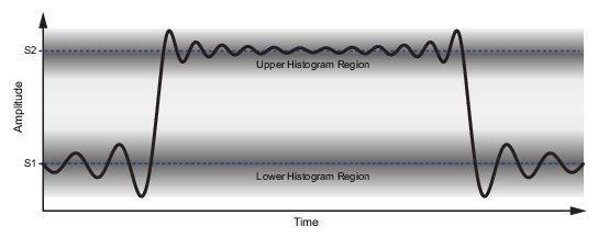
When the pulse level type is set to AUTO a histogram algorithm method is used for determining the high and low state levels as described in the IEEE Standard for Pulses, Transitions, and Related Waveforms (181-2011), Section 5.2.1. The trace data is taken as input and the amplitudes are operated on in terms of dBm units. The trace data is converted into a histogram where the number of bins is determined by a fixed bin width of 0.01 across the total range of values in the trace data (trace max to trace min). In other words, each trace point amplitude results in an incremented "count" in the histogram bin that corresponds to the amplitude range in which that amplitude falls. To find the high and low state levels, the resulting histogram is split into an "upper" and "lower" histogram where the former consists of all the bins that correspond to the upper 50% range of amplitudes, and the latter the lower 50% range. Then the high state is determined to be the mode of the upper histogram, i.e. the amplitude corresponding to the histogram bin with the highest count. The low state is similarly determined to be the mode of the lower histogram.
If the count of either mode is not greater than at least 1% of the total number of points in the trace data input, then the histogram is recreated using a bin width that is ten times larger. This process of regenerating the histogram with larger a bin width is repeated until the mode of the histogram is at least 1% of the total number of points. This means that the best case resolution of the resulting high state and low state is 0.01 dBm (the starting bin width), and depending on how much the state levels fluctuate, the resolution can fall back to 0.1 dBm, 1 dBm, and so on.
Finding High and Low Reference Levels
When the pulse level type is set to USER, the user determines the high and low state levels and enters the level using the USER TOP (S2) and USER BOTTOM (S1) settings.
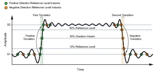
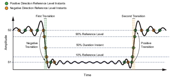
Transitions are contiguous regions of a waveform that connect, either directly or via intervening transients, two state occurrences that are consecutive in time but are occurrences of different states. To find the transition, begin with a filtered list of reference level instants that contain only those that cross the low or high reference levels. Each reference level instant in the list has a corresponding index and direction (e.g. the trace index immediately before the amplitude crossing the reference level, and direction indicating whether the trace crosses from above to below the reference level or vice versa).
This filtered list of instants is sorted in ascending index order. Then all positive and negative transitions (between the high/low reference levels) are found by searching for consecutive instants in the filtered list that both have the same direction. The waveform is defined to be in the "high state" if it exceeds the 90% reference level and in the "low state" if it drops below the 10% reference level. This is the chosen alternative rather than using the state upper/lower boundaries (which the IEEE standard says is optional).
Finding Pulse Duration and Period
The pulse duration is determined by using the positive and negative transitions as describe above to check if it is a valid pulse. If so, then any pulse duration reference levels (50%) are verified to exist within the positive/negative transition. This reference level determines the starting and ending period of the pulse. The duration is just the difference between the ending point and the starting point.
The pulse period also first determines that we have a valid pulse from the positive and negative transitions. Unlike the pulse duration measurement, the pulse period must have the pulse repeat, or a pulse train, to have a measurement. There should be at least 3 transitions in the 50% reference level to produce a valid measurement. The period is the distance between the starting level of the first pulse and the starting level for the second pulse.
Finding the Wave Average
The wave average is determined by averaging the power levels of all points within all complete periods that are available on the trace. To determine where to start and stop, the number of transitions is used to determine if there is at least one full period. The system returns "nan" if there is not a full period. Otherwise, the starting point for this measurement is the beginning of the first transition and the end point is the beginning of the transition of the last full period.
For instance, a trace with six transitions has some quantity of points before the first transition followed by two full periods, then followed by less than one full period. Once the start and end of all the complete periods have been found, all points between them are summed together and divided by the total number of points used in the measurement.
Finding Trace Average
The trace average is the exponential average of all the points in the trace. Unlike the wave average, it is not constrained to full pulses.
Finding the Pulse Average
The pulse average is the average of the points in the high state of the pulse (typically those points above the 90% reference line). This only applies to positive pulses. If there is no positive pulse, then no measurement is returned.
Finding the Pulse Center Instant and Repetition Frequency
The Pulse repetition frequency is determined from the inverse of the pulse period (1/pulse period) as a frequency value. The pulse center instant is determine by taking the pulse duration (50%) start time and adding the pulse duration midpoint, which is one-half of the pulse duration (pulse duration/2).
Finding the Pulse Peak
The pulse peak is the maximum value in a waveform after a positive transition. If there is no positive transition, the peak amplitude of the overall waveform is returned.
Finding the Pulse Tilt
The pulse tilt measures the distortion of a waveform state where the overall slope of the state is essentially constant and other than zero. The slope may be of either polarity and is calculated for either negative or positive pulses. A complete pulse (with at least two transitions) is needed to ensure that there is a waveform state for which tilt can be measured. If there is enough trace data within the waveform state, the first and last 25% of samples where overshoot distortion is most likely to occur is removed. The slope of the remaining 50% of state trace data is then calculated using the least squares method, and the tilt is calculated by multiplying the slope by the number of trace points in the state.
Finding the Wave Amplitude
The wave amplitude is found by subtracting the amplitude of the lower state level from the amplitude of the upper state level in dB units.
Finding the Peak to Wave Average
The peak to wave average is found by subtracting the wave average from the pulse peak in terms of dB. This requires the wave average to have a valid value, so there must be at least one full period for a measurement.
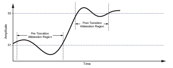
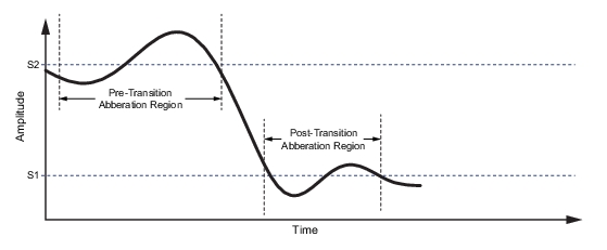
Finding the Pre- and Post-Transition Aberration Region
The pre-transition aberration region is determined to be the region of the trace before the last state crossing before the first transition, and with a width equal to three times the duration of the first transition. It is upper bounded by the available trace data before the transition. The post-transition aberration region is the region beginning at the first state crossing past the first transition, and ending at three times the transition duration or at the beginning of the next transition, whichever comes first.
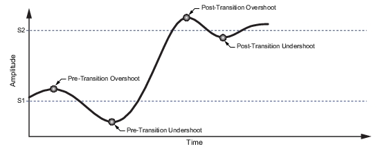
Positive Pulse Aberration Regions
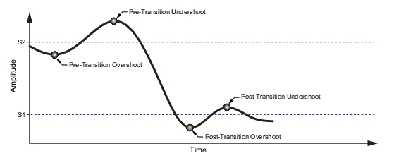
Negative Pulse Aberration Regions
Finding the Overshoot and Undershoot of Each Aberration Region
The overshoot and undershoot of each region are calculated by taking the difference between the maximum and minimum trace value of each aberration region and the local state level. Local state level being (Low = pre-transition → High = post-transition) in a positive transition, and (High = pre-transition → Low = post-transition) in a negative transition.
Positive Pulse Overshoot and Undershoot
Negative Pulse Overshoot and Undershoot
Tips for Improving Pulse Measurement Results
• Set the reference level as close to the top of the trace as possible.
• Use trace averaging.
• For custom or irregular pulses, use a user defined top reference level (S2) instead of auto detection.
• Use single sweep and sweep once buttons to take measurements one at a time.