The automatic measurement process analyzes the captured signal data in the following sequence:
1. Approximately 500 samples of the waveform (equivalent to one screen width) are scanned to determine the maximum and minimum sample amplitudes.
2. The difference between the maximum and minimum sample values is calculated and stored as the Signal Amplitude.
3. The Transition Threshold is computed as one-half the sum of the maximum and minimum sample amplitudes.
4. The processor locates each crossing of the Transition Threshold.
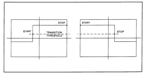
5. Starting at the left edge of the screen, the processor classifies each Transition threshold crossing according to whether it is positive-going (– +) or negative-going (+ –). Because the signal is repetitive, only three transitions are needed to classify the waveform as shown in Table: Transition Threshold.
6. If the signal is Type 0, (No crossings detected) no measurements can be performed and the routine is terminated, pending the next reload of the data buffers.
7. The process locates the bottom amplitude (baseline) using the IEEE histogram method. A histogram is generated for all samples in the lowest 12.8 dB range of sample values. The range is subdivided into 64 power levels of 0.2 dB each. The histogram is scanned to locate the power level with the maximum number of crossings. This level is designated the baseline amplitude. If two or more power value have equal counts, the lowest is selected.
8. The process follows a similar procedure to locate the top amplitude (top line). The power range for the top histogram is 5 dB and the resolution is 0.02 dB, resulting in 250 levels. The level-crossing histogram is computed for a single pulse, using the samples which exceed the transition threshold. If only one transition exists in the buffer (Types 2 and 3), the process uses the samples that lie between the edge of the screen and the transition threshold as shown in Figure: Time Interpolation. For a level to be designated the top amplitude, the number of crossings of that level must be at least 1/16 the number of pixels in the pulse width; otherwise, the peak value is designated the top amplitude.
9. The process establishes the proximal, mesial, and distal levels as a percentage of the difference between top amplitude and bottom amplitude power. The percentage can be calculated on a power or voltage basis. The proximal, mesial, and distal threshold values are user settable from 1% to 99%, with the restriction that the proximal < mesial < distal. Normally, these values will be set to 10%, 50%, and 90%, respectively.
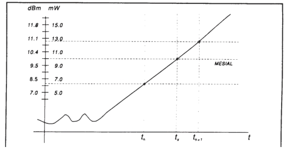
10. The process determines horizontal position, in pixels, at which the signal crosses the mesial value. This is done to a resolution of 0.1 pixel, or 1/5000 of the screen width. Ordinarily, the sample values do not fall precisely on the mesial line, and it is necessary to interpolate between the two nearest samples to determine where the mesial crossing occurred as shown in Figure: Time Interpolation.
Time Interpolation
Mesial Value
Item
dBm
mW
Mesial
value
10.0
Sample n
8.0
6.3
Sample n+1
11.0
12.6
The interpolated crossing time, tx, is calculated from:
tx = tn + (Pmes – Pn)/(Pn+1– Pn )
where P is in watts and n is the number of the sampling interval, referenced to the trigger event. For this example:
tx = tn+(10.0 –6.3)/(12.6 – 6.3)
tx = tn+0.6
The processor computes the rise and/or fall times of waveforms that meet the following conditions: The waveform must have at least one usable edge (Step 2 through Step 7).
• The signal peak must be at least 13 dB greater than the minimum sample value.
• The rise time is defined as the time between the proximal and distal crossings (– +).
The fall time is defined as the time between the distal and proximal crossings (+ –).
If no samples lie between the proximal and distal values for either edge (rise or fall), the risetime for that edge is set to 0 seconds.
The processor calculates the output values according to the following definitions as described in Table: Definitions.: