Inter- and Intra-Trace Math and Operand Setup Menus
INTER-TRACE MATH Menu
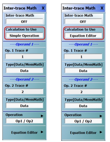
This menu allows operand setting and then mathematical comparisons between a user-defined trace 1 (one) and trace 2 (two). The two traces values can be added together, subtracted from each other, multiplied, or divided. If using Equation Editor, multiple traces can be operated upon.
• MAIN | Display | DISPLAY | Inter-trace Math | INTER-TRACE MATH | Operation | INTRA-TRACEOP
INTRA-TRACE OP. (INTRA TRACE OPERATIONS) Menu
See below for button function descriptions.
INTRA TRACE OP. Menu Button Selection Group
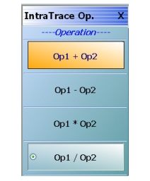
The four (4) buttons of the INTRA TRACE OPERATIONS menu form a button selection group where the selection of any one (1) button de-selects the other three (3) buttons.
Operation Area
Op1 + Op2 (Operand Plus)
The trace value assigned to Operand 1 is added to the trace value assigned to Operand 2.
Op1 – Op2 (Operand Subtraction)
The trace value assigned to Operand 2 is subtracted from the trace value assigned to Operand 1.
Op1 * Op2 (Operand Multiplication)
The trace value assigned to Operand 1 is multiplied times the trace value assigned to Operand 2.
Op1 / Op2 (Operand Division)
The trace value assigned to Operand 1 is divided by the trace value assigned to Operand 2.
EQUATION EDITOR Dialog Box
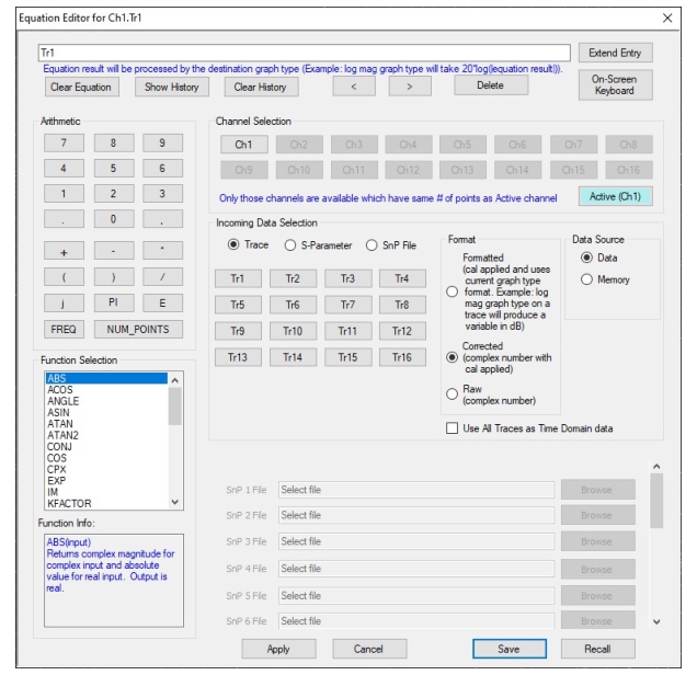
The Equation Editor allows a much more complete set of operations between trace data sets (and S-parameter sets) than does the Simple Operation inter-trace math. The main dialog is shown in Figure: Inter-Trace Math Equation Editor and consists of a selection of functions, input variables (traces and s-parameters in various formats) and scalar entry along with some editing tools.
A central concept is that the entire equation is based on complex vectors of length equal to the number of points. Scalars (real or complex) can be used throughout but, where necessary, will be automatically vectorized (same value at each position in a vector of length equal to the number of points).
MAIN | Display | DISPLAY | Inter-Trace Math | INTER-TRACE MATH | Equation Editor | EQUATION EDITOR FOR TRx Dialog Box
Inter-Trace Math Equation Editor
Note
Syntax errors will be flagged if parentheses are not used to resolve precedence problems (e.g., Tr1 * –T2 will not be accepted but Tr1 * (–Tr2) will be).
Equation Editor Contents:
Clear Equation Button
• Clears equation entry bar above.
Show History Button
• Clicking button opens window showing equation history (equation controls are hidden). Clicking again returns user to equation controls.
Clear History Button
• Clears equation history.
< and > Buttons
• Moves the cursor either left or right within the equation entry bar.
Extend Entry Button
• Clicking Extend Entry opens a larger text edit field for directly typing in longer or more complex equations.
Function Selection Pane
Following are descriptions of the functions supported (the output of the function is complex unless otherwise noted).
• ABS() – Complex magnitude for complex input and absolute value for real input. Output is real.
• ACOS() – Arccosine, radian output. This will accept complex arguments and uses the standard branch cut.
• ANGLE() – Phase of complex input; radian output. Output is real.
• ASIN() – Arcsine, radian output. This will accept complex arguments and uses the standard branch cut.
• ATAN() – Arctangent, radian output. This will accept complex arguments and uses the standard branch cut.
• ATAN2() – Arctangent with the ability to properly resolve quadrants. The argument is complex and it is internally split into real and imaginary components with sign checking. Radian output
• CONJ() – Conjugate
• COS() – Cosine, radian input. Note that this function will accept complex inputs and treat them as such. Commonly one would use this function only with a formatted trace set up for phase and then multiplied by pi/180 to convert to radians.
• CPX(a,b) – Complex equivalent taking 2 real inputs; output is a+jb. If the inputs are complex, the real part of each is taken prior to combination into a new complex variable.
• EXP() – Exponential
• IM() – Imaginary part of a complex input. Output is real.
• MAG() – Magnitude accepting complex input (same as ABS). Output is real.
• MAX() – Maximum value of the MAGNITUDE of the variable selected. (Note that this updates only after a sweep completes so there may be a one sweep delay until the value propagates to a plotted equation). Output is real.
• MAX_HOLD() Accumulates maximum value of the MAGNITUDE of the argument sweep-to-sweep. The process is reset by clearing the equation or turning inter-trace math off. (Note that this updates only after a sweep completes so there may be a one sweep delay until the value propagates to a plotted equation). Output is real.
• MEAN() – Average value in a complex sense; (Note that this updates only after a sweep completes so there may be a one sweep delay until the value propagates to a plotted equation)
• MEDIAN() – Median value of the MAGNITUDE of the argument; (Note that this updates only after a sweep completes so there may be a one sweep delay until the value propagates to a plotted equation). Output is real.
• MIN() – Minimum value of the MAGNITUDE of the argument; (Note that this updates only after a sweep completes so there may be a one sweep delay until the value propagates to a plotted equation). Output is real.
• MIN_HOLD() – Accumulates maximum value of the MAGNITUDE of the argument sweep-to-sweep. The process is reset by clearing the equation or turning inter-trace math off. (Note that this updates only after a sweep completes so there may be a one sweep delay until the value propagates to a plotted equation). Output is real.
• MRKX() – Readout of active maker on entered trace, x-value. If no marker is on, a 0 will be returned. If more than one marker is on, the active marker will be used. Output is real. Since this function relies on a trace marker value, the argument can be ONLY a trace and not a function involving a trace.
• MRKY() – Readout of active maker on entered trace, y-value. If no marker is on, a 0 will be returned. If more than one marker is on, the active marker will be used. Since this function relies on a trace marker value, the argument can be ONLY a trace and not a function involving a trace.
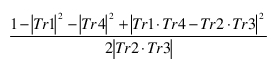
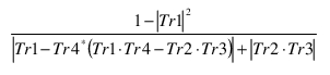
• MU: mu stability factor accepting four complex inputs (generally representing S11, S12, S21, and S22).
• MU(Tr1,Tr2,Tr3,Tr4) produces:
Equation 27‑2.
(where the * denotes conjugate)
Output is real.
• PHASE() – Same as ANGLE but degree output. Output is real.
• POW(z,n) – Raises a complex variable z to the nth power. n is a scalar.
• RE() – Returns real part of a complex input. Output is real.
• REWRAP() – Rewraps phase of a complex variable when range was truncated (often by a power function). The calculation is based on slope of low frequency data.
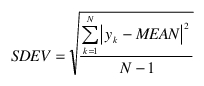
• SDEV() – Standard deviation of input data. This is evaluated only at sweep completion so there may be a one sweep delay for values to propagate to a displayed equation.
• This calculation is based on the equation below where N is the number of points. Output is real.
Equation 27‑3.
• SIN() – Sine; (Note that this function will accept complex inputs and treat them as such). Commonly one would use this function only with a formatted trace set up for phase and then multiplied by pi/180 to convert to radians.
• SQRT() – Square root; standard branch cut.
• SUBSET(a,b,Trace) – Accepts a vector argument (Trace) and extracts elements from point indices 'a' to 'b' of the Trace vector. Note that for the point indices 'a' and 'b', the first point of the sweep is point 0. 'Trace' refers to any vector representing a current data or memory trace (like the arguments for other functions) or a vector resulting from other computations.
• TAN() – Tangent. (Note that this function will accept complex inputs and treat them as such). Commonly one would use this function only with a formatted trace set up for phase and then multiplied by pi/180 to convert to radians.
• XAXISARRAY() – Generates the vector corresponding to the current sweep variable. Output is real.
Channel Selection Pane
Data (and memory and processed results) from other channels may be used in the calculation for the active channel. Specified parameters from the highlighted channel will be used in the equation. All channels being used are required to have the same number of sweep points. Default selection is Active channel.
Incoming Data Selection Pane
Format
• Formatted
If Formatted is selected, the current graph type format will be used so the vector may be purely real. Cal will be applied and will use current graph format.
• Raw and Corrected
If the trace selection format is selected as Raw or Corrected, the variable will enter the equation as a linear complex number (either with or without calibration applied; Note that receiver calibrations are applied to all).
• Data Source Selections
• Data – Current trace data
• Memory– Data stored in trace memory
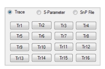
Trace Radio Button
• Select enables buttons for selections of traces Tr1 through Tr16:
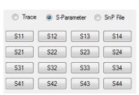
S-Parameter Radio Button
• Select enables buttons for selections of S-Parameters:
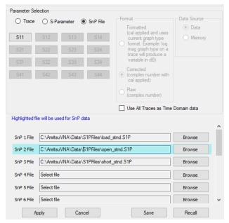
SnP File Radio Button
• Select enables fields for browsing to and selecting SnP files. The highlighted file will be used for SnP data. A maximum of 16 SnP files can be loaded; they are shared per system.
Arithmetic Keypad Area
• Constant π (PI) is available and the 'j' button is used for entering complex scalars. The scientific notation exponent marker 'E' is also available (e.g., 1E9 for 1,000,000,000).
Use All Traces as Time Domain Data
• If the time domain checkbox is selected, all traces and parameters will be processed into time domain in the background if they are not already displayed that way. Lowpass Processing will be used if the current frequency list supports it, but otherwise Bandpass Process will be used. Trace time domain parameters will be used which may be at default if not already configured. It is recommended to configure desired variables in time domain so the results are predictable. See the Measurement Guide (10410-00218) for more information.
Save Equation
• Saves existing equation to a designated location as a .eqn file.
Recall Equation
• Recalls an existing equation .eqn file from its saved location.
Note
Trace memory and trace math can be used as the incoming variables.