To verify the performance of the transmission feed line system and analyze typical problems, three types of line sweeps can be performed:
• Return Loss
• Cable Loss
• Distance-To-Fault
Note
Anritsu recommends using a phase-stable test port cable, attached to the Site Master RF port. Calibrate at the open end of the cable.
Return Loss/VSWR Measurement
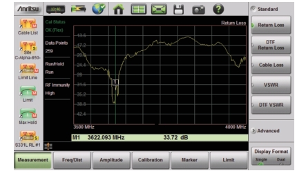
This is a measurement made when the antenna is connected at the end of the transmission line. It provides an analysis of how the various components of the system are interacting.
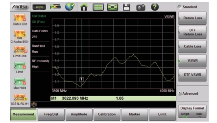
Return Loss measures the reflected power of the system in decibels (dB). This measurement can also be taken in the Standing Wave Ratio (SWR) mode, which is the ratio of voltage peaks to voltage valleys caused by reflections.
Antenna Return Loss Trace
Same Antenna Trace in VSWR
The following describes the main steps to follow when making Return Loss or VSWR measurements.
1. Press the Measurement main menu key and select Return Loss or VSWR.
2. Press the Freq/Dist main menu key and enter the start and stop frequencies.
3. Press the Amplitude main menu key and enter the top and bottom values for the display or press Fullscale.
4. Press the Calibration main menu key and perform a calibration of the instrument. Anritsu suggests using a phase-stable test port cable. See Calibration for details.
5. Connect the Site Master to the Device Under Test using the calibrated phase-stable test port cable.
6. Press the Marker main menu key and set the appropriate markers as described in Markers.
7. Press the Limit main menu key to enter and set the limit line as described in Limit Lines.
8. Press Save (7) then Save to save the measurement to memory. Refer to Save File for details on setting the save location.
Cable Loss Measurement
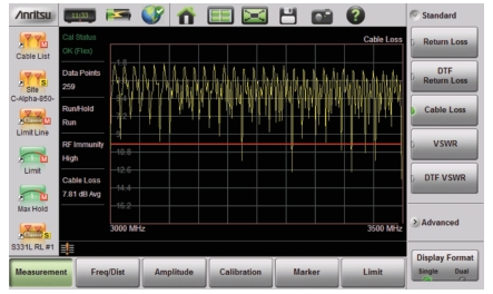
Cable loss sweep is made when a short is connected at the end of the transmission line. This insertion loss test allows analysis of the signal loss through the transmission line and identifies problems in the system. High insertion loss in the feed line or jumpers can contribute to poor system performance and loss of coverage.
Different transmission lines have different losses, depending on frequency and distance. The higher the frequency or longer the distance, the greater the loss. This measurement returns the energy absorbed, or lost, by the transmission line in dB/meter or dB/ft. The average cable loss of the frequency range is displayed on the screen in the measurement settings summary area.
Cable Loss Measurement
The following describes the main steps to follow when making Cable Loss measurements.
1. Press the Measurement main menu key and select Cable Loss.
2. Press the Freq/Dist key and enter start and stop frequencies.
3. Press the Amplitude main menu key and enter top and bottom values for the display or press Full Scale.
4. Press the Calibration main menu key to start calibration of the instrument. Anritsu suggests using a phase-stable test port cable. See Calibration for details.
5. Connect the Site Master to the Device Under Test using the calibrated phase-stable test port cable.
6. Press the Limit main menu key to enter and set the limit line as described in Limit Lines. This limit line is used only for visual reference and not a pass/fail guide. The pass/fail determination is based on the average cable loss.
7. Press Save (7), then Save to save the measurement to memory. Refer to Save File for details on setting the save location.
DTF Measurement
Distance-To-Fault (DTF) measurements are made with the antenna disconnected and replaced with a 50 Ω precision load at the end of the transmission line. This measurement allows analysis of the various components of the transmission feed line system in the DTF mode.
This measurement reveals the precise fault location of components in the transmission line system. This test helps to identify specific problems in the system, such as connector transitions, jumpers, kinks in the cable or moisture intrusion.
The first step is to measure the distance of a cable. This measurement can be made with an open or a short connected at the end of the cable. The peak indicating the end of the cable should be between 0 dB and 5 dB. An open or short should not be used when DTF is used for troubleshooting the system because the open/short will reflect most of the RF energy from the Site Master and the true value of a connector might be misinterpreted or a good connector may look like a failing connector.
A 50 Ω load is the best termination for troubleshooting DTF problems because it will be 50 Ω over the entire frequency range. The antenna can also be used as a terminating device but the impedance of the antenna will change over different frequencies since the antenna is typically only designed to have 15 dB or better return loss in the passband of the antenna.
DTF measurement is a frequency domain measurement and the data is transformed to the time domain. The distance information is obtained by analyzing how much the phase is changing when the system is swept in the frequency domain. Frequency selective devices such as TMAs (Tower Mounted Amplifiers), duplexers, filters, and quarter wave lightning arrestors change the phase information (distance information) if they are not swept over the correct frequencies. Care needs to be taken when setting up the frequency range whenever a TMA is present in the path.
Using DTF Aid
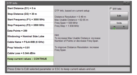
Because of the nature of the measurement, maximum distance range and distance resolution are dependent upon the frequency range and number of data points. DTF Aid (Freq/Distance > Distance > DTF Aid) shown in Figure: DTF Aid explains how the parameters are related.
DTF Aid
If the cable is longer than DMax, the only way to improve the horizontal range is to reduce the frequency span or to increase the number of data points. Similarly, the distance resolution is inversely proportional to the frequency range and the only way to improve the distance resolution is to widen the frequency span.
Note
When determining the frequency range, consider all in-line frequency selective devices.
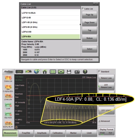
Cable List
Selecting the cable type is critical for accurate DTF measurements. Incorrect propagation velocity (PV) values affect the distance accuracy, and inaccurate cable attenuation values affect the accuracy of the amplitude values. The Site Master S331L is equipped with a cable list (Freq/Dist > DTF Setup > Cable List) including most of the common cables currently used. Once the correct cable has been selected, the instrument will update the propagation velocity and the cable attenuation values to correspond with the cable. For setups with several different cable types, choose the main feeder cable.
For cables not on the list, select NONE and manually enter the Prop Velocity and Cable Loss in DTF Aid or the DTF Setup submenu.
Custom Cables can be created and uploaded to the instrument using Line Sweep Tools (LST). Instructions for using the LST Cable Editor are available in the software Help menu. The latest version of LST is available from the Anritsu web site: http://www.anritsu.com/.
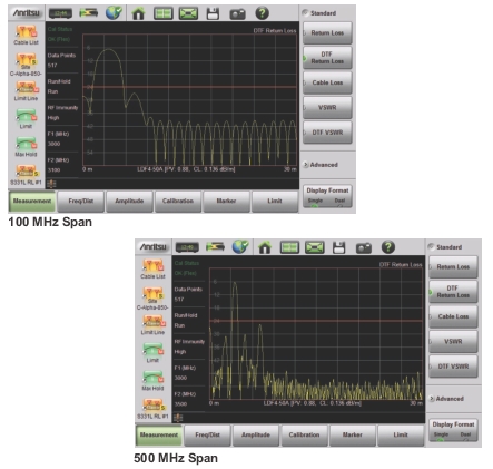
The name, propagation velocity, and cable loss of the selected cable are displayed below the trace window during distance measurements (Measurement > DTF Return Loss or DTF VSWR) as shown in Figure: Cable List Selection Displayed Under Graticule.
Cable List Selection Displayed Under Graticule
Distance Resolution
Distance resolution is the Site Master’s ability to separate two closely spaced discontinuities. If the resolution is 5 meters and there are two faults 3 meters apart, the Site Master will not be able to show both faults until the resolution is improved by widening the frequency span.
Distance Resolution (m) = 1.5 x 10⁸ x PV / ΔF (in Hz)
with Rectangular Windowing applied.
Figure: DTF Measurements at 100 MHz vs. 500 MHz is an example of the same DTF measurement with a 100 MHz span vs. a 500 MHz span. The increased span provides additional detail that there may be several unique issues with the first 10 meters of the cable. This detail was not available in the narrower span.
DTF Measurements at 100 MHz vs. 500 MHz
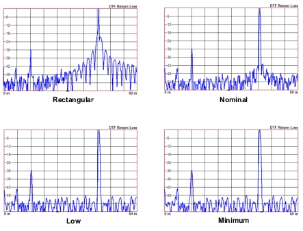
Windowing
The theoretical requirement for inverse FFT is for the data to extend from zero frequency to infinity. Side lobes appear around a discontinuity because the spectrum is cut off at a finite frequency. Windowing reduces the side lobes by smoothing out the sharp transitions at the beginning and the end of the frequency sweep. As the side lobes are reduced, the main lobe widens, thereby reducing the resolution.
In situations where a small discontinuity may be close to a large one, side lobe reduction windowing helps to reveal the discrete discontinuities. If distance resolution is critical, then reduce the windowing for greater signal resolution.
If two or more signals are very close to each other, then spectral resolution is important. In this case, use Rectangular Windowing for the sharpest main lobe (the best resolution).
In summary:
• Rectangular windowing provides best spatial distance resolution for revealing closely spaced events, but the side lobes close to any major event (large reflection) may mask smaller events which are close to the major event. Excellent choice if multiple faults of similar amplitudes close together are suspected.
• Nominal Side Lobe windowing provides very good suppression of close-in side lobes, but compromises spatial distance resolution compared to Rectangular. Closely spaced events may appear as a single event, often non-symmetrical in shape. Excellent overall choice for most typical antenna system sweeps.
• Low Side Lobe windowing provides excellent suppression of close-in side lobes but spatial distance resolution is worse than Nominal Side Lobe. The additional suppression of side lobes may be useful in locating very small reflection events further away from large events. It is not often used for field measurements.
• Minimum Side Lobe windowing provides highest suppression of side lobes but worst spatial distance resolution. Can be useful for finding extremely small events spaced further apart than the distance resolution. Again, not typically used for field measurements.
Effects of Windowing on a Sample Trace
DMax (Maximum Usable Distance)
DMax is the maximum horizontal distance that can be analyzed. The Stop Distance cannot exceed DMax. If the cable is longer than DMax, DMax needs to be improved by increasing the number of data points or lowering the frequency span (ΔF). Note that the data points can be set to 130, 259, 517, 1033, or 2065 (Sweep> Data Points).
DMax = (Datapoints – 1) x Distance Resolution
The following describes the main steps to follow when making DTF Return Loss or DTF VSWR measurements.
1. Press the Measurement main menu key and select DTF Return Loss or DTF VSWR.
2. Press the Freq/Dist main menu key.
3. Press the Distance submenu key and then select DTF Aid. Use the touchscreen, rotary knob, or Up/Down arrow keys to navigate through all the DTF parameters.
a. Highlight a parameter in the DTF Aid table to edit, then press Edit or Enter to display a parameter for editing.
b. Edit all required parameters and then highlight Keep current values -- CONTINUE and press Enter.
Note
If Stop Distance is greater than DMax, increase the number of data points.
4. Connect a phase-stable Test Port cable to the RF Out/Reflect In connector on the Site Master. Press the Calibration main menu key to start calibration of the instrument. Refer to Calibration for details.
5. Connect the Site Master to the Device Under Test using the calibrated phase-stable test port cable.
Example 1 – DTF with a Short to Measure Cable Length
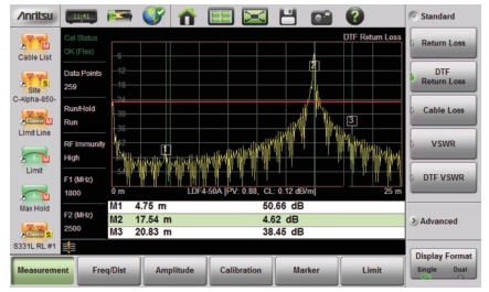
To measure the length of a cable, DTF measurements can be made with an open or a short connected at the end of the cable. The peak indicating the end of the cable should be between 0 dB and 5 dB. In Figure: DTF Return Loss with a Short at the End of the Cable (20.5 m) the cable end is at 20.5 meters.
The cable end was found by selecting Marker 3 (Marker > Select M(1-8) > M3) then using searching for the trace peak (Marker > Marker Search > Marker to Peak).
DTF Return Loss with a Short at the End of the Cable (20.5 m)
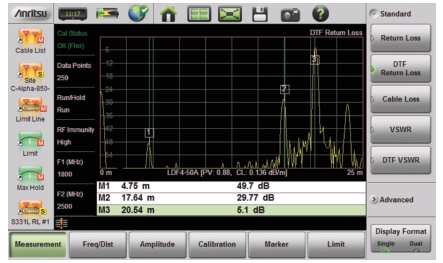
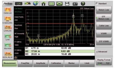
The Distance-To-Fault transmission line test verifies the performance of the transmission line assembly and its components and identifies the fault locations in the transmission line system. This test determines the return loss value of each connector pair, cable component and cable to identify the problem location. This test can be performed in the DTF-Return Loss or DTF-VSWR mode. Typically, for field applications, the DTF-Return Loss mode is used. Figure: DTF Return Loss Measurement (Antenna at 20.83 m) shows the failure with the antenna still attached.
Failing DTF Return Loss Measurement (Load at 20.83 m)
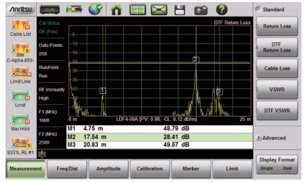
The jumper connector at 17.5 m was found to be loose and dirty. After cleaning and tightening to specification, another DTF measurement showed that the connector now passed the carrier 25 dB specification, indicated by the limit line (Figure: Passing DTF Return Loss Measurement (Load at 20.83 m)).
Passing DTF Return Loss Measurement (Load at 20.83 m)