This section describes the various Cable and Antenna Analyzer measurements. Note that not all measurements are supported in all instruments. Some of the measurements are option dependent. Please refer to your product’s technical data sheet for the list of supported options.
MEASURE Menu
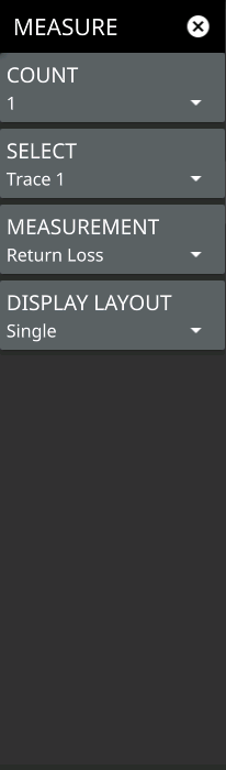
From the main menu select MEASURE > MEASUREMENT menu to select one of the desired measurements.
MEASURE Menu
COUNT:
Select the display format of single (1) or horizontal split (2).
SELECT:
Select the desired active trace for setting up measurement parameters.
MEASUREMENT:
Select one of the desired measurement type from the following list:
• Transmission (2-Port): Verifies the performance of tower-mounted amplifiers, and duplexers, and antenna isolation between two sectors. Refer to Transmission (2-port) Measurement (Option 21).
• TDR Ohm: Measures the mismatch of the transmission line impedance against distance. Refer to TDR OHM (Option 3) Measurement.
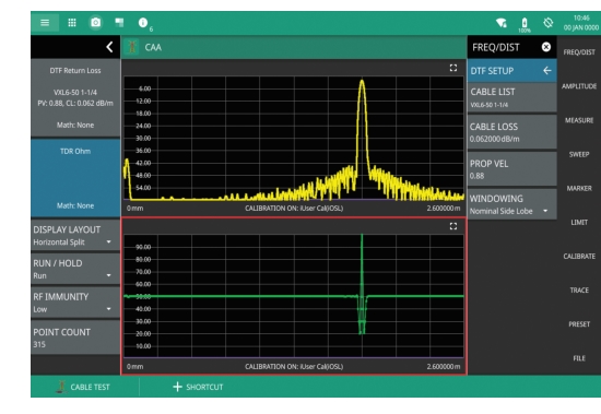
Select either one measurement trace (Single) or two measurement traces (Horizontal Split). In horizontal split display format, the active measurement trace is framed with a red border and the measurement trace card in the status panel will have a blue background. You can touch either trace to make it the active trace.
Return Loss Measurement
This is a measurement made when the antenna is connected at the end of the transmission line. It provides an analysis of how the various components of the system are interacting.
Return Loss is used to characterize RF components and systems. The Return Loss indicates how well the system is matched by taking the ratio of the reflected signal to the incident signal, and measuring the reflected power in dB.
Return Loss Measurement
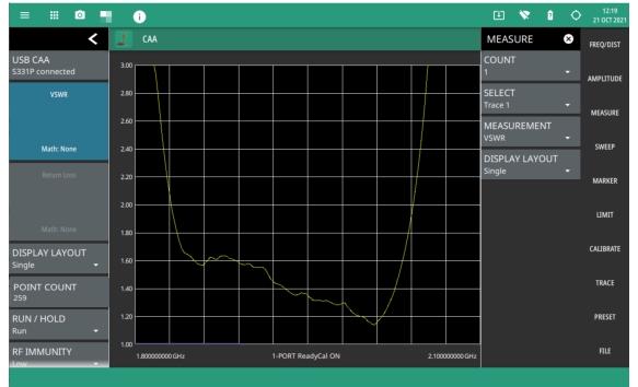
VSWR Measurement
This is a measurement made when the antenna is connected at the end of the transmission line. It provides an analysis of how the various components of the system are interacting.
VSWR is a ratio of voltage peaks to voltage valleys and allows you to view the impedance match. This measurement is similar to return loss, but is the ratio of voltage peaks to voltage valleys caused by reflections.
VSWR Measurement
To make return loss or VSWR measurements:
1. Select MEASURE on the main menu and then select MEASUREMENT > Return Loss or VSWR.
2. Select FREQ/DIST on the main menu, then enter the start and stop frequencies.
3. Select AMPLITUDE on the main menu, then enter the top and bottom power levels for the display, or press FULL SCALE.
4. For the most accurate results, press CALIBRATION on the main menu and perform a manual calibration of the instrument. Refer to .
Alternatively, you can skip this step and the instrument will automatically apply the factory calibration (1-Port ReadyCal ON).
5. Connect the instrument/S331P to the device under test.
6. Select MARKER on the main menu and then set the appropriate markers as described in Setting Up Markers.
7. Select LIMIT on the main menu and then set up limit lines as described in Setting Up Limit Lines.
8. To save the measurement data or setup to a file, press FILE > SAVE AS..., and then select the location and file type you want to save. Refer to Saving a Measurement for details on saving measurement data or setups to a file.
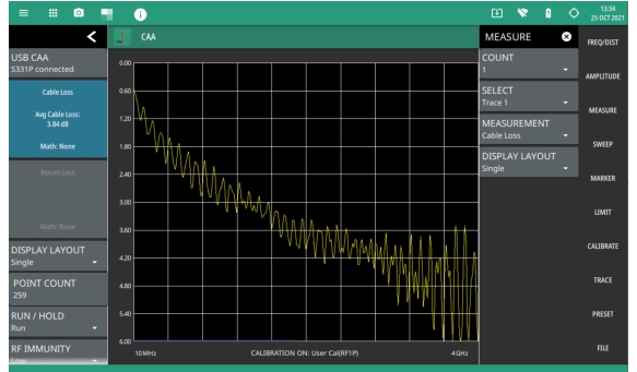
Cable Loss Measurement
The cable loss measurement verifies the signal attenuation level of a cable. Cable loss sweep is made when a short is connected at the end of the transmission line. This insertion loss test allows analysis of the signal loss through the transmission line and identifies problems in the system. High insertion loss in the feed line or jumpers can contribute to poor system performance and loss of coverage.
Different transmission lines have different losses, depending on frequency and distance. The higher the frequency or longer the distance, the greater the loss. This measurement returns the energy absorbed, or lost, by the transmission line in dB/meter or dB/ft. The average cable loss of the frequency range is displayed on the trace card. Figure: Cable Loss Measurement is a cable loss measurement example.
Cable Loss Measurement
To make a cable loss measurement:
1. Select MEASURE on the main menu and then select MEASUREMENT > Cable Loss.
2. Select FREQ/DIST and enter the start and stop frequencies.
3. Select AMPLITUDE, then enter the top and bottom power levels for the display or press FULL SCALE.
4. For the most accurate results, press CALIBRATION on the main menu and perform a manual calibration of the instrument. Refer to .
Alternatively, you can skip this step and the instrument will automatically apply the factory calibration (1-PORT ReadyCal ON).
5. Connect the instrument/S331P to one end of the cable under test, then connect a short to the other end of the cable under test.
6. Select MARKER on the main menu and then set the appropriate markers as described in Setting Up Markers.
7. Select LIMIT on the main menu and set the limit line as described in Setting Up Limit Lines. This limit line is used only for visual reference and not a pass/fail guide. The pass/fail determination is based on the average cable loss shown in the trace card.
8. To save the measurement data or setup to a file, press FILE > SAVE AS..., and then select the location and file type you want to save. Refer to Saving a Measurement for details on saving measurement data or setups to a file.
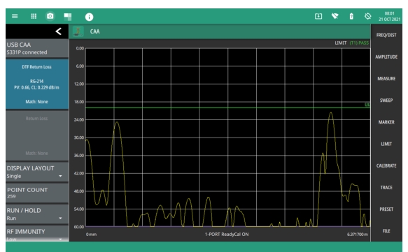
DTF Return Loss and DTF VSWR Measurement
Distance-to-Fault (DTF) measurements are made with the antenna disconnected and replaced with a 50 Ω precision load at the end of the transmission line. This measurement allows analysis of the various components of the transmission feed line system in the DTF mode.
This measurement reveals the precise fault location of components in the transmission line system. This test helps to identify specific problems in the system, such as connector transitions, jumpers, kinks in the cable or moisture intrusion.
The first step is to measure the distance of a cable. This measurement can be made with an open or a short connected at the end of the cable. The peak indicating the end of the cable should be between 0 dB and 5 dB. An open or short should not be used when DTF is used for troubleshooting the system because the open/short will reflect most of the RF energy from the RF test port and the true value of a connector might be misinterpreted or a good connector may look like a failing connector.
A 50 Ω load is the best termination for troubleshooting DTF problems because it will be 50 Ω over the entire frequency range. The antenna can also be used as a terminating device, but the impedance of the antenna will change over different frequencies since the antenna is typically only designed to have 15 dB or better return loss in the passband of the antenna.
DTF measurement is a frequency domain measurement and the data is transformed to the time domain. The distance information is obtained by analyzing how much the phase is changing when the system is swept in the frequency domain. Frequency selective devices such as TMAs (tower mounted amplifiers), duplexers, filters, and quarter wave lightning arrestors change the phase information (distance information) if they are not swept over the correct frequencies. Care needs to be taken when setting up the frequency range whenever a TMA is present in the path.
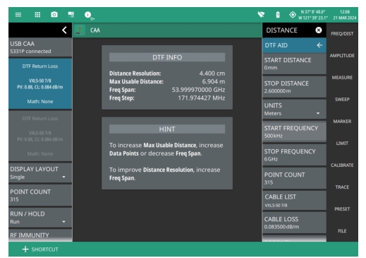
DTF Aid
Because of the nature of the measurement, maximum distance range and distance resolution are dependent upon the frequency range and number of data points. DTF Aid (FREQ/DIST > DISTANCE > DTF AID) shown in Figure: DTF Aid explains how the parameters are related.
DTF Aid
The maximum usable distance may be extended by either increasing the number of sweep data points or by reducing the current frequency span. Distance resolution is inversely proportional to the frequency span and may be increased by setting a wider frequency span. Windowing can also affect distance resolution. For the best distance resolution, select Rectangular Windowing.
Note
When determining the frequency range, consider all in-line frequency selective devices.
Cable List
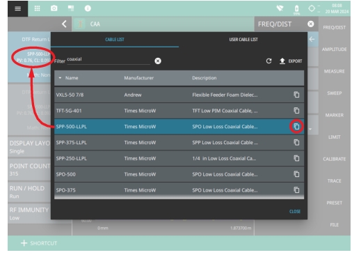
Selecting the cable type is critical for accurate DTF measurements. Incorrect propagation velocity values (PV) affect the distance accuracy, and inaccurate cable attenuation values affect the accuracy of the amplitude values. The Cable and Antenna Analyzer is equipped with a cable list (FREQ/DIST > DTF SETUP > CABLE LIST) including most of the common cables currently used. Once the correct cable has been selected, the instrument will update the propagation velocity and the cable attenuation values to correspond with the cable. For setups with several different cable types, choose the main feeder cable.
For cables not on the list, select NONE and manually enter the propagation velocity (PROP VEL) and cable loss in DTF AID or the DTF SETUP menu.
The name, propagation velocity, and cable loss of the selected cable are displayed in the status panel’s trace card during distance measurements (MEASURE > MEASUREMENT > DTF Return Loss or DTF VSWR) as shown in Figure: Cable List Selection.
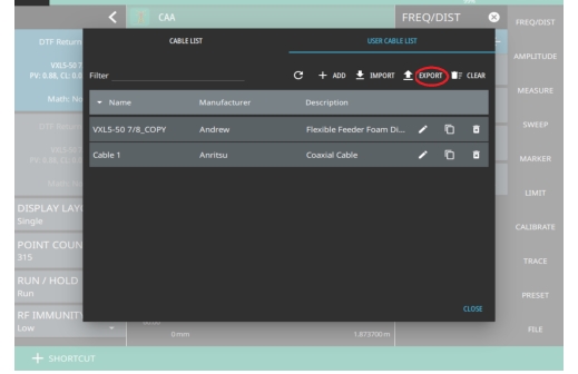
The cable list window has the following options:
• Enter a keyword in FILTER field found in the top of the list to search for a specific cable of interest, for e.g. coaxial.
• Select copy icon to add a copy of the selected cable to the USER CABLE LIST.
• Select EXPORT button on the top right corner of the cable list window to save the cable to the instrument’s internal memory.
• Select refresh icon to refresh the cable list.
Cable List Selection
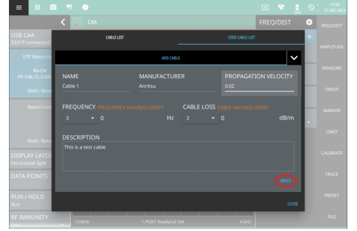
User Cable List
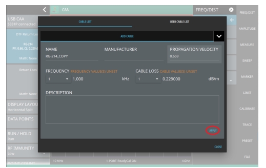
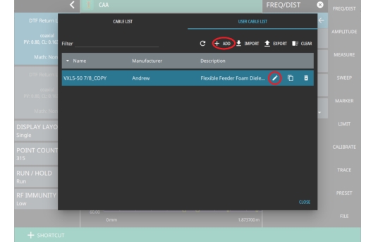
To add a custom user cable to the user cable list follow the instructions below:
2. Go to USER CABLE LIST to view the newly added cable. If required select the edit icon to change the name of the cable as shown in as shown in Figure: User Cable List - Edit.
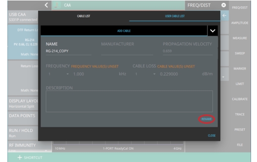
User Cable List - Edit
3. Enter the name of the cable and select RENAME button at the bottom of the window. Note that you can only rename the cable from this window.
Distance resolution is the Field Master Series’s ability to separate two closely spaced discontinuities. If the resolution is 5 meters and there are two faults 3 meters apart, the Field Master Series will not be able to show both faults until the resolution is improved by widening the frequency span.
Distance Resolution (m) = 1.5 x 10⁸ x PV / ΔF (in Hz)
with Rectangular Windowing applied.
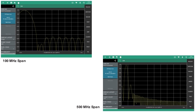
Figure: DTF Measurements at 100 MHz vs. 500 MHz (Field Master Series) is an example of the same DTF measurement with a 100 MHz span vs. a 500 MHz span. The increased span provides additional detail that there may be several unique issues with the first 10 meters of the cable. This detail was not available in the narrower span.
DTF Measurements at 100 MHz vs. 500 MHz (Field Master Series)
Windowing
The theoretical requirement for inverse FFT is for the data to extend from zero frequency to infinity. Side lobes appear around a discontinuity because the spectrum is cut off at a finite frequency. Windowing reduces the side lobes by smoothing out the sharp transitions at the beginning and end of the frequency sweep. The main lobe widens as the side lobes are reduced, thus reducing the resolution.
In situations where a small discontinuity may be close to a large one, side lobe reduction windowing helps to reveal the discrete discontinuities. If distance resolution is critical, then reduce the windowing for greater signal resolution.
If two or more signals are very close to each other, then spectral resolution is important. In this case, use Rectangular Windowing for the sharpest main lobe (the best resolution).
To select the windowing type, follow this key sequence:
FREQ/DIST > DISTANCE > DTF AID > WINDOWING >
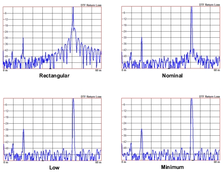
• Rectangular windowing provides best spatial distance resolution for revealing closely spaced events, but the side lobes close to any major event (large reflection) may mask smaller events which are close to the major event. Excellent choice if multiple faults of similar amplitudes close together are suspected.
• Nominal Side Lobe windowing provides very good suppression of close-in side lobes, but compromises spatial distance resolution compared to Rectangular. Closely spaced events may appear as a single event, often non-symmetrical in shape. Excellent overall choice for most typical antenna system sweeps.
• Low Side Lobe windowing provides excellent suppression of close-in side lobes, but spatial distance resolution is worse than Nominal Side Lobe. The additional suppression of side lobes may be useful in locating very small reflection events further away from large events. It is not often used for field measurements.
• Minimum Side Lobe windowing provides highest suppression of side lobes but worst spatial distance resolution. Can be useful for finding extremely small events spaced further apart than the distance resolution. Again, not typically used for field measurements.
Effects of Windowing on a Sample Trace
Maximum Usable Distance
The maximum horizontal distance that can be analyzed is displayed in the DTF Aid Info dialog, of which the stop distance cannot exceed. If the cable is longer than this max distance, the setup needs to be improved by increasing the number of data points or lowering the frequency span. Note that the data points can be set to 130, 259, 517, 1033, or 2065 (SWEEP > DATA POINTS).
Max Distance = (Datapoints – 1) x Distance Resolution
To make DTF Return Loss or DTF VSWR measurements:
1. Select MEASURE > MEASUREMENT and select DTF Return Loss or DTF VSWR.
2. Select the FREQ/DIST > DISTANCE > DTF AID, then select a setup parameter and follow the on-screen guidance in the DTF Aid Info dialog.
3. Repeat the above step above to edit more parameters until the setup is complete.
4. For the most accurate results, press CALIBRATION on the main menu and perform a manual calibration of the instrument. Refer to .
Alternatively, you can skip this step and the instrument will automatically apply the factory calibration (1-Port ReadyCal ON).
5. Connect the instrument to the device under test.
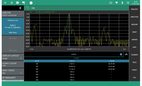
Example 1 – DTF with a Short to Measure Cable Length
To measure the length of a cable, DTF measurements can be made with an open or a short connected at the end of the cable. Provided you have selected the appropriate cable type from the Cable List, the peak indicating the end of the cable should be 0 dB or a value close to zero. In Figure: DTF Return Loss with a Short at the End of the Cable, the cable end is at 20.5 meters.
The cable end was found by selecting Marker 1, then searching for the trace peak. (MARKER > MARKER SEARCH > Peak)
DTF Return Loss with a Short at the End of the Cable
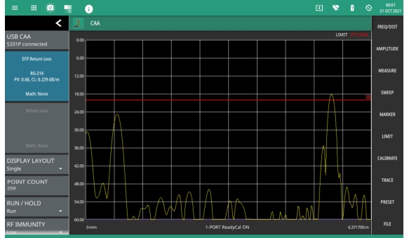
The Distance-to-Fault transmission line test verifies the performance of the transmission line assembly and its components and identifies the fault locations in the transmission line system. This test determines the return loss value of each connector pair, cable component and cable to identify the problem location. This test can be performed in the DTF Return Loss or DTF VSWR mode. Typically, for field applications, the DTF Return Loss mode is used. Figure: Failing DTF Return Loss Measurement (Antenna) shows the failure with the antenna still attached.
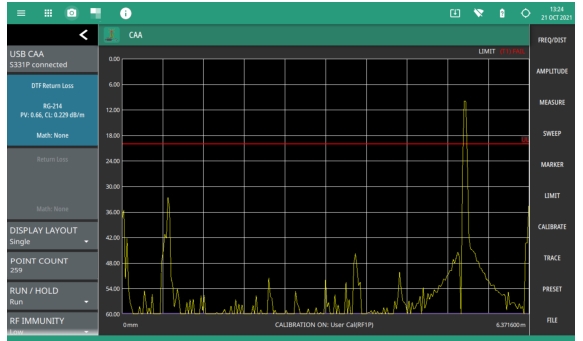
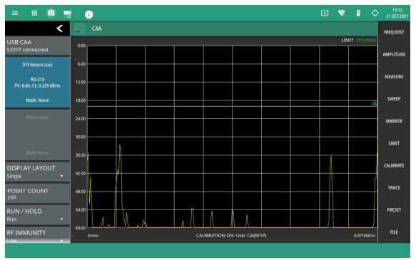
The jumper connector at the antenna end of the cable was found to be loose and dirty. After cleaning and tightening to specification, another DTF measurement showed that the connector now passed the carrier 20 dB specification, indicated by the limit line (Figure: Passing DTF Return Loss Measurement (Load)).
The Smith Chart is a graphical tool for plotting impedance data versus frequency. It converts the measured reflection coefficient data into complex impedance data and displays it in a manner that makes the Smith Chart a useful tool for determining and tuning input match. Markers can be used to read the real and imaginary parts of the complex impedance. See the example in Figure: Smith Chart Measurement. This impedance plot reveals which matching elements (capacitance, inductance) are necessary to match a device under test to the reference impedance (50 ohms).
Smith Chart Measurement
To make a smith chart measurement:
1. Select MEASURE on the main menu and then select MEASUREMENT > Smith Chart.
2. Select FREQ/DIST and enter the start and stop frequencies.
3. For the most accurate results, press CALIBRATION on the main menu and perform a manual calibration of the instrument. Refer to .
Alternatively, you can skip this step and the instrument will automatically apply the factory calibration (1-PORT ReadyCal ON).
4. Connect the RF test port of the instrument to the device under test.
5. Select MARKER on the main menu and then set the appropriate markers as described in Setting Up Markers.
6. To save the measurement data or setup to a file, press FILE > SAVE AS..., and then select the location and file type you want to save. Refer to Saving a Measurement for details on saving measurement data or setups to a file.
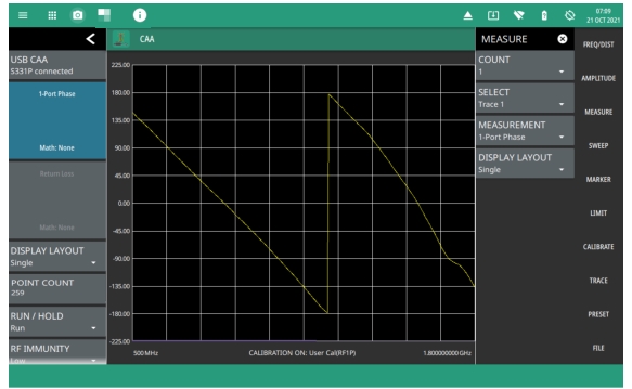
1-Port Phase Measurement
The Cable and Antenna Analyzer can display the phase of the reflection measurements at the RF port. The Phase display range is from –450 degrees to +450 degrees. The 1-port phase measurement is most useful when making relative measurements (comparing the phase of one device to the phase of another) by utilizing the Trace Math function (Trace – Memory).
1-Port Phase Measurement
1. Select MEASURE on the main menu and then select MEASUREMENT > 1-Port Phase.
2. Select FREQ/DIST and enter the start and stop frequencies.
3. Select AMPLITUDE, then enter the maximum and minimum angles for the display or press FULL SCALE.
4. For the most accurate results, press CALIBRATION on the main menu and perform a manual calibration of the instrument. Refer to .
Alternatively, you can skip this step and the instrument will automatically apply the factory calibration (1-PORT ReadyCal ON).
5. Connect the instrument/S331P to the device under test.
6. Select MARKER on the main menu and then set the appropriate markers as described in Setting Up Markers.
7. Select LIMIT on the main menu and set the limit line as described in Setting Up Limit Lines. This limit line is used only for visual reference and not a pass/fail guide. The pass/fail determination is based on the average cable loss shown in the trace card.
8. To save the measurement data or setup to a file, press FILE > SAVE AS..., and then select the location and file type you want to save. Refer to Saving a Measurement for details on saving measurement data or setups to a file.
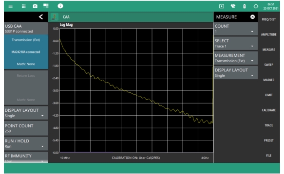
Transmission (USB Sensor) Measurement
The Transmission measurement is used to measure the loss (or gain) in dB of a device. This measurement requires that one port of the device be connected directly (or through a test port cable) to the RF port of the S331P. The second port of the device connects to an external USB sensor. To make more accurate cable loss measurements, especially for cables with more than 10 dB of loss, you can use the transmission measurement with an external sensor. For this measurement, connect the cable under test to the RF port of the S331P and connect a USB power sensor to the other end of the cable. USB extenders can be used for long cable runs.
This measurement gives accurate results of cable loss up to 30 dB. This is a scalar measurement, providing only magnitude data (no phase) and, therefore, does not use vector error correction for its calibration steps. Instead, it uses a sensor reference calibration. Figure: External Sensor Transmission Measurement is a cable loss transmission measurement example with an external power sensor, which can be compared to the example shown in Figure: Cable Loss Measurement.
External Sensor Transmission Measurement
For best results when performing both transmission and return loss measurements on the same cable, the return loss should be measured with a good-quality termination at the end of the cable.
Note
For a list of external USB sensors that are supported by the Cable and Antenna Analyzer for transmission measurements, see your instrument’s Technical Data Sheet.
Only a supported USB power sensor is necessary to make Transmission (USB sensor) measurements, the purchase of Option 19, High Accuracy Power Meter (HIPM) is not required.
Table: Cable and Antenna Measurement Overview presents a summary of the typical measurements and required cable end tool. The typical values are for general information purposes. The carriers will provide final values in the acceptance testing specification.
Cable and Antenna Measurement Overview
Measurement
Mode
End Tool
Marker
TYPICAL PASS/FAIL MEASUREMENTS
Pass/Fail Test of Cable & Connectors
Freq Return Loss or Freq, SWR
Load
Peak
Pass/Fail Test of System Including Antenna
Freq Return Loss or Freq, SWR
Antenna
Peak
Frequency Range of Antenna
Freq Return Loss or Freq, SWR
Antenna
Valley
Cable Loss
Freq Cable Loss
Short or Open
Peak & Valley
Cable Loss (High Accuracy)
Freq Cable Loss (Open and Short) / 2 using trace memory function
Short and Open
Peak
Return Loss
Freq Return Loss
Load
Peak
TROUBLESHOOTING MEASUREMENTS
Cable Length
DTF Return Loss or DTF SWR
Short or Open
Peak
Good Cable & Connectors
DTF Return Loss or DTF SWR
Load
Peak
Good System Including Antenna
DTF Return Loss or DTF SWR
Antenna
Peak
To set up a, external USB sensor transmission measurement:
1. Select MEASURE on the main menu and then select MEASUREMENT > Transmission (USB Sen).
2. Select FREQ/DIST and enter the start and stop frequencies.
3. Select AMPLITUDE, then enter the top and bottom power levels for the display or press FULL SCALE.
4. For the most accurate results, press CALIBRATION on the main menu and perform a manual calibration of the instrument. Refer to .
Alternatively, you can skip this step and the instrument will automatically apply the factory calibration (1-PORT ReadyCal ON).
5. Connect the instrument/S331P and power sensor to the device or cable under test.
6. Select MARKER on the main menu and then set the appropriate markers as described in Setting Up Markers.
7. Select LIMIT on the main menu and set the limit line as described in Setting Up Limit Lines. This limit line is used only for visual reference and not a pass/fail guide. The pass/fail determination is based on the average cable loss shown in the trace card.
8. To save the measurement data or setup to a file, press FILE > SAVE AS..., and then select the location and file type you want to save. Refer to Save File for details on saving measurement data or setups to a file.
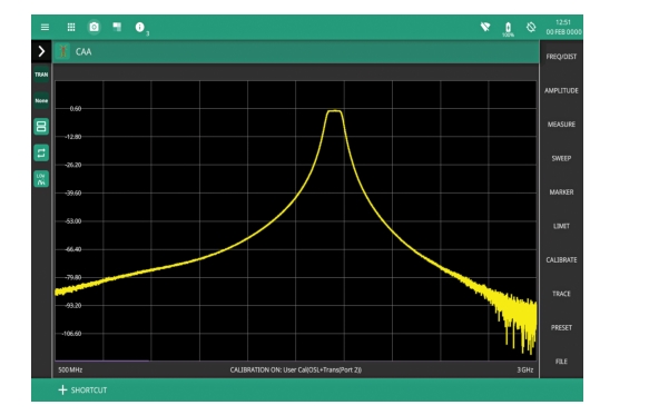
Transmission (2-port) Measurement (Option 21)
The 2-port transmission measurement is used to verify the performance of tower-mounted amplifiers, and duplexers, and to verify antenna isolation between two sectors. The excellent dynamic range makes it suitable for repeaters as well. The second port is a selective receiver which provides up to 100 dB dynamic range which makes it possible to test the band pass filters common on many networks.
Both high and low power settings are available. The high-power setting delivers approximately 0 dBm power at the RF out port, ideal for antenna isolation measurements and duplexers. When making measurements of a Tower Mounted Amplifier, Anritsu recommends to use the low-power setting (approximately –40 dBm). This will ensure that the RF In port is not over-powered and that the measurements are made in the linear region of the amplifier. This measurement is only available on Site Master instruments.
Transmission Measurement
To set up a, 2-port transmission measurement:
1. Select MEASURE on the main menu and then select MEASUREMENT > Transmission.
2. Select FREQ/DIST and enter the start and stop frequencies.
3. Select AMPLITUDE, then enter the top and bottom power levels for the display or press FULL SCALE.
4. For the most accurate results, press CALIBRATION on the main menu and perform a manual calibration of the instrument. Refer to .
Alternatively, you can skip this step and the instrument will automatically apply the factory calibration (1-PORT ReadyCal ON).
5. Select MARKER on the main menu and then set the appropriate markers as described in Setting Up Markers.
6. Select LIMIT on the main menu and set the limit line as described in Setting Up Limit Lines. This limit line is used only for visual reference and not a pass/fail guide. The pass/fail determination is based on the average cable loss shown in the trace card.
7. To save the measurement data or setup to a file, press FILE > SAVE AS..., and then select the location and file type you want to save. Refer to Saving a Measurement for details on saving measurement data or setups to a file.
Time Domain Reflectometry (TDR) Measurements (Option 3)
Time Domain Reflectometry (TDR) is a technique that measures and displays the impedance of a network (cable, filter etc) over time.
A TDR measurement shows impedance against distance, with a normal 50 ohm line running across the center of the display. Different causes of reflections such as open circuits, short circuits, kinks to the outer cable conductor and water ingress will cause characteristic changes to the transmission line impedance. This in turn helps identify the cause of the fault and accelerates the repair process.
TDR OHM (Option 3) Measurement
TDR Ohm measurement involves using TDR to analyze the impedance or characteristic impedance of a transmission line or cable. TDR instruments provide valuable information about impedance mismatches, cable faults, and variations in characteristic impedance.
TDR OHM Measurement
TDR Linear (Option 3) Measurement
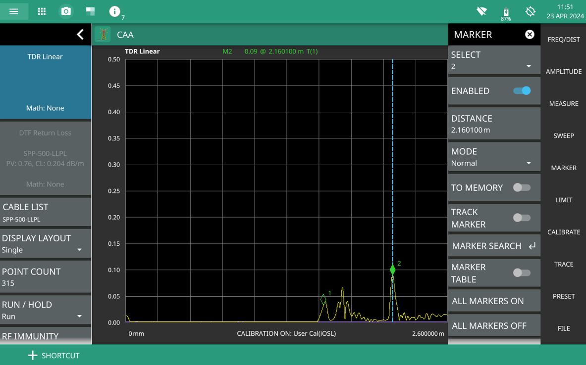
The TDR Linear measurement is a linear representation of the return loss (or gain) in dB of a device in time domain. The time domain transform of the underlying s-parameter is integrated into a step response (and presumably plotted on a linear scale).
TDR Linear Measurement
To set up TDR measurements:
1. Select MEASURE on the main menu and then select MEASUREMENT > TDR Ohm/TDR Linear.
2. Select FREQ/DIST and enter the start and stop frequencies.
3. Select AMPLITUDE, then enter the top and bottom power levels for the display or press FULL SCALE.
4. For the most accurate results, press CALIBRATION on the main menu and perform a manual calibration of the instrument. Refer to .
Alternatively, you can skip this step and the instrument will automatically apply the factory calibration (1-PORT ReadyCal ON).
5. Select MARKER on the main menu and then set the appropriate markers as described in Setting Up Markers.
6. Select LIMIT on the main menu and set the limit line as described in Setting Up Limit Lines. This limit line is used only for visual reference and not a pass/fail guide. The pass/fail determination is based on the average cable loss shown in the trace card.